Chapter 10 Problems
of “Modern Compressible Flow With Historical Perspective”, Third Edition, John D. Anderson Jr
[1]:
import pint
import pygasflow
from pygasflow.solvers import *
import numpy as np

ureg = pint.UnitRegistry()
# use "~P" to format units with unicode
ureg.formatter.default_format = "~"
# let pygasflow knows which UnitRegistry to use
pygasflow.defaults.pint_ureg = ureg
# dictionary results offers improved code readability
pygasflow.defaults.solver_to_dict = True

# shorcuts for conveniance
kg = ureg.kg
K = ureg.K
degC = ureg.degC
J = ureg.J
m = ureg.m
atm = ureg.atm
Pa = ureg.pascal
sec = ureg.s
deg = ureg.deg
Q_ = ureg.Quantity

gamma = 1.4
R = 287.05 * J / (kg * K)
P 10.1
[2]:
M_inf = 2
theta_c = 15 * deg
p1 = 1 * atm
T1 = 290 * K
rho1 = (p1 / (R * T1)).to("kg/m**3")
[3]:
shock = conical_shockwave_solver(M_inf, "theta_c", theta_c)
shock.show()
key        quantity
--------------------------
mu         Mu                  2.00000000
mc         Mc                  1.70686796
theta_c    theta_c [deg]      15.00000000
beta       beta [deg]         33.91469753
delta      delta [deg]         4.57913858
pr         pd/pu               1.28614663
dr         rhod/rhou           1.19636349
tr         Td/Tu               1.07504671
tpr        p0d/p0u             0.99837756
pc_pu      pc/pu               1.56629305
rhoc_rhou  rho_c/rhou          1.37718896
Tc_Tu      Tc/Tu               1.13731165
(a)
[4]:
beta = shock["beta"]
beta
[4]:
33.91469752764406 deg
(b)
[5]:
p1 = 1 * atm
T1 = 290 * K
rho1 = (p1 / (R * T1)).to("kg / m**3")
rho1
[5]:
1.2171975325697193 kg/m3
[6]:
p2 = shock["pr"] * p1
p2
[6]:
1.2861466346503097 atm
[7]:
T2 = shock["tr"] * T1
T2
[7]:
311.763546391508 K
[8]:
rho2 = shock["dr"] * rho1
rho2
[8]:
1.4562106866511302 kg/m3
[9]:
M2 = shockwave_solver("mu", M_inf, "theta", shock["delta"])["md"]
M2
[9]:
np.float64(1.8362269055556388)
(c)
[10]:
pc = shock["pc_pu"] * p1
pc
[10]:
1.5662930485508126 atm
[11]:
Tc = shock["Tc_Tu"] * T1
Tc
[11]:
329.8203785583531 K
[12]:
rhoc = shock["rhoc_rhou"] * rho1
rhoc
[12]:
1.6763110037955304 kg/m3
P 10.2
for a cone
[28]:
from pygasflow.interactive.diagrams import ConicalShockDiagram
ConicalShockDiagram().show_figure()
[14]:
from pygasflow.shockwave import max_theta_c_from_mach
from scipy.optimize import bisect

M_inf = 2
theta_c = 15 * deg

def func(M, theta_target):
    _, theta_c_max, _ = max_theta_c_from_mach(M, gamma)
    return theta_c_max - theta_target

M = bisect(func, a=1+1e-05, b=M_inf, args=(theta_c.magnitude))
M
[14]:
1.1191542916165758
Detachment happens for \(M < 1.1191542916165758\).
for a wedge
[29]:
from pygasflow.interactive.diagrams import ObliqueShockDiagram
ObliqueShockDiagram().show_figure()
[16]:
from pygasflow.shockwave import max_theta_from_mach
from scipy.optimize import bisect

M_inf = 2
theta_c = 15 * deg

def func(M, theta_target):
    theta_max = max_theta_from_mach(M, gamma)
    return theta_max - theta_target

M = bisect(func, a=1+1e-05, b=M_inf, args=(theta_c.magnitude))
M
[16]:
1.6142820055343785
Detachment happens for \(M < 1.6142820055343785\).
P 10.3
[17]:
theta_c = 15 * deg
p_inf = 1 * atm
T_inf = 290 * K
rho_inf = (p_inf / (R * T_inf)).to("kg/m**3")
\[C_{D} = \frac{D}{q_{inf} A_{b}}\]
[18]:
M_inf = np.linspace(1.5, 7, 10)
shock = conical_shockwave_solver(M_inf, "theta_c", theta_c)
shock.show()
key        quantity
--------------------------
mu         Mu                  1.50000000     2.11111111     2.72222222     3.33333333     3.94444444     4.55555556     5.16666667     5.77777778     6.38888889     7.00000000
mc         Mc                  1.27072629     1.80016926     2.29347872     2.75349994     3.17963867     3.57165457     3.93004456     4.25599373     4.55121833     4.81778887
theta_c    theta_c [deg]      15.00000000    15.00000000    15.00000000    15.00000000    15.00000000    15.00000000    15.00000000    15.00000000    15.00000000    15.00000000
beta       beta [deg]         45.03026984    32.39931734    26.84465529    23.79812548    21.92451816    20.68444478    19.81985693    19.19291942    18.72400453    18.36431587
delta      delta [deg]         2.80388765     4.96695670     6.87069448     8.33449443     9.42354578    10.23421622    10.84493203    11.31219851    11.67548013    11.96228586
pr         pd/pu               1.14722014     1.32613297     1.59632397     1.94402320     2.36398123     2.85413484     3.41372871     4.04253583     4.74053666     5.50778528
dr         rhod/rhou           1.10299119     1.22258193     1.39250825     1.59417198     1.81538994     2.04704461     2.28202585     2.51482448     2.74131739     2.95858072
tr         Td/Tu               1.04009910     1.08469865     1.14636590     1.21945639     1.30218923     1.39427095     1.49592026     1.60748229     1.72929142     1.86163090
tpr        p0d/p0u             0.99973580     0.99771208     0.98966824     0.97077703     0.93817677     0.89178335     0.83377611     0.76761276     0.69709000     0.62567597
pc_pu      pc/pu               1.37807332     1.61529077     1.92632241     2.30655383     2.75631763     3.27636708     3.86738084     4.52989659     5.26432413     6.07097059
rhoc_rhou  rho_c/rhou          1.25732469     1.40755796     1.59253566     1.80127311     2.02582645     2.25905044     2.49474539     2.72783422     2.95440559     3.17164250
Tc_Tu      Tc/Tu               1.09603615     1.14758384     1.20959452     1.28051311     1.36058922     1.45032932     1.55021064     1.66062020     1.78185560     1.91414089
[19]:
pc = shock["pc_pu"] * p_inf
pc
[19]:
| Magnitude | [1.3780733219251478 1.615290767532153 1.9263224149410585 2.3065538292079126 2.7563176271935834 3.2763670844886 3.8673808351142953 4.52989659160189 5.264324126219128 6.070970594438352] |
|---|---|
| Units | atm |
[20]:
# NOTE: I'm going to use sympy + pint together in order to check dimensions as I compute things
import sympy as sp
# chord length
c = Q_(sp.symbols("c", positive=True, real=True), m)
# length of the oblique side
l = c / sp.cos(theta_c.to("radian").magnitude)
# radius of the cone
r = l * sp.sin(theta_c.to("radian").magnitude)
[21]:
# surface area of the base of the cone
Ab = sp.pi * r**2
Ab
[21]:
0.0717967697244908*pi*c**2 m2
[22]:
# surface area of the cone
Ac = sp.pi * r * l
Ac
[22]:
0.277401416484059*pi*c**2 m2
[23]:
D = pc * Ac * sp.cos(theta_c.to("radian").magnitude) - p_inf * Ab
D = D.to("N")
D
[23]:
| Magnitude | [30139.8167444177*pi*c**2 36580.2589879646*pi*c**2 45024.7532616738*pi*c**2 55348.017878665*pi*c**2 67559.0833707194*pi*c**2 81678.4011339047*pi*c**2 97724.3960492736*pi*c**2 115711.666986197*pi*c**2 135651.339242044*pi*c**2 157551.752073121*pi*c**2] |
|---|---|
| Units | N |
[24]:
a_inf = np.sqrt(gamma * R * T_inf).to("m/s")
V_inf = a_inf * M_inf
V_inf
[24]:
| Magnitude | [512.0743842451016 720.6972815301431 929.3201788151845 1137.9430761002259 1346.5659733852672 1555.1888706703085 1763.8117679553502 1972.4346652403917 2181.057562525433 2389.680459810474] |
|---|---|
| Units | m/s |
[25]:
q_inf = rho_inf * V_inf**2 / 2
q_inf
[25]:
| Magnitude | [159586.87499999994 316108.9814814815 525607.800925926 788083.3333333334 1103535.5787037036 1471964.5370370366 1893370.2083333335 2367752.592592593 2895111.689814815 3475447.4999999995] |
|---|---|
| Units | kg/(m s2) |
[26]:
Cd = D / (q_inf * Ab)
Cd = Cd.to("")
Cd
[26]:
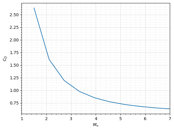
[2.63050136760627 1.61177730228564 1.19312139720313 0.978194067556690 0.852692619429496 0.772867376823472 0.718890179395168 0.680668925858093 0.652610200866927 0.631404393868821]
[27]:
import matplotlib.pyplot as plt
fig, ax = plt.subplots()

ax.plot(M_inf, Cd.magnitude)
ax.set_xlabel(r"$M_{\infty}$")
ax.set_ylabel(r"$C_{D}$")
ax.set_xlim(1, M_inf.max())
ax.grid(visible=True, which="both")
ax.grid(which="major", linestyle="--", color="0.8")
ax.grid(which="minor", linestyle=":", color="0.9")
ax.minorticks_on()
plt.show()
[ ]: