Common functionalities
- pygasflow.common.sound_speed(*args)[source]
Compute the sound speed.
There are two modes of operations:
sound_speed(gamma, R, T): compute the sound speed for a perfect gas. It also hold for thermally perfect as well as calorically perfect gases.sound_speed(gas): provide a Cantera’sSolutionobject, from which the parameters will be retrieved.
Alias of this function:
speed_of_sound.- Parameters:
- args
- gammafloat or array_like
Specific heats ratio. Default to 1.4. Must be \(\gamma > 1\).
- Rfloat or array_like
Specific gas constant [J / (kg * K)]
- Tfloat or array_like
Temperature of the gas [K].
- gasct.Solution, optional (second mode of operation)
A Cantera’s
Solutionobject from which the quantities will be retrieved.
- Returns:
- afloat or array_like
Sound speed [m / s]
Examples
Compute the speed of sound of air at 300K. First mode of operation, providing gamma, R, T:
>>> from pygasflow.common import sound_speed
>>> sound_speed(1.4, 287, 300)
np.float64(347.18870949384285)
Compute the speed of sound of air at multiple temperatures:
>>> sound_speed(1.4, 287, [300, 500])
array([347.18870949, 448.21869662])
Compute the sound speed in N2 at 300K and 1atm:
>>> import cantera as ct
>>> gas = ct.Solution("gri30.yaml")
>>> gas.TPX = 300, ct.one_atm, {"N2": 1}
>>> sound_speed(gas)
np.float64(353.1256637274762)
- pygasflow.common.pressure_coefficient(Mfs, param_name='pressure', param_value=None, stagnation=False, gamma=1.4)[source]
Compute the pressure coefficient of a compressible flow. For supersonic flows, the pressure coefficient downstream of the shockwave is returned.
- Parameters:
- Mfsfloat or array_like
Free stream Mach number. If float, list, tuple is given as input, a conversion will be attempted. Must be Mfs > 0. If Mfs > 1 (supersonic case), it corresponds to the Mach number upstream of the shock wave.
- param_namestr, optional
Name of the ratio. It can be:
'm': specify the local Mach number.'velocity': specify the ratio between the local speed and the free stream speed, u / ufs.'pressure': specify the ratio between the local pressure and the total pressure, p / pt.'pressure_fs': specify the ratio between the local pressure and the free stream pressure, p / pfs.
Default to
'pressure'.- param_valuefloat or None, optional
The value of the parameter. For Mfs < 1 either
param_valuemust be different thanNone, orstagnation=Truemust be set.- stagnationbool, optional
False: (default value) compute the local pressure coefficient. For subsonic Mfs,param_nameandparam_valuemust be provided.True: compute the pressure coefficient at the stagnation point. In this case, onlyMfsis required. If Mfs > 1, isentropic flow is assumed from just downstream of the shockwave to the stagnation point.
- gammafloat, optional
Specific heats ratio. Default to 1.4. Must be \(\gamma > 1\).
- Returns:
- cpndarray
Pressure coefficient.
References
“Basic of Aerothermodynamics”, by Ernst H. Hirschel
“Hypersonic Aerothermodynamics” by John J. Bertin
Examples
Pressure coefficients at the stagnation point:
>>> from pygasflow.common import pressure_coefficient
>>> Minf = [0.01, 0.1, 0.5, 1, 5, 10]
>>> pressure_coefficient(Minf, stagnation=True)
array([1.000025  , 1.0025025 , 1.06407222, 1.27561308, 1.80876996,
       1.83167098])
Pressure coefficients at the stagnation point, by specifying a parameter:
>>> pressure_coefficient(Minf, "velocity", 0)
array([1.000025  , 1.0025025 , 1.06407222, 1.27561308, 1.80876996,
       1.83167098])
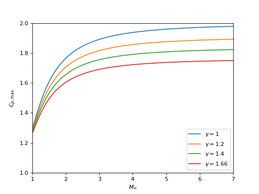
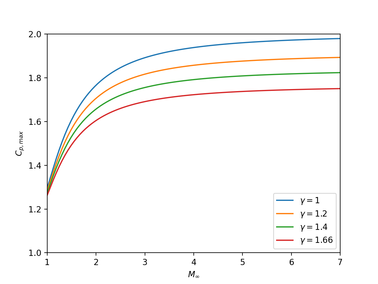
Variation of the stagnation-pressure coefficient with the free stream Mach number and the ratio of specific heats:
from pygasflow import pressure_coefficient
import matplotlib.pyplot as plt
import numpy as np

M_inf = np.linspace(1, 7, 100)
gammas = [1 + 1e-05, 1.2, 1.4, 1.66]
fig, ax = plt.subplots()
for g in gammas:
    cp = pressure_coefficient(M_inf, stagnation=True, gamma=g)
    ax.plot(M_inf, cp, label=r"$\gamma = %s$" % (1 if np.isclose(g, 1) else g))

ax.legend(loc="lower right")
ax.set_xlim(M_inf.min(), M_inf.max())
ax.set_ylim(1, 2)
ax.set_xlabel(r"$M_{\infty}$")
ax.set_ylabel("$C_{p, max}$")
plt.show()
(
Source code,png,hires.png,pdf)