Nozzles
This module contains classes to build/visualize nozzle geometries, which can
then be used with De_Laval_Solver.
Each nozzle has a certain number of editable parameters and read-only parameters. By changing an editable parameter, the nozzle class will immediatly recompute all other parameters.
Converget-Divergent Conical
- class pygasflow.nozzles.cd_conical.CD_Conical_Nozzle(Ri=0.4, Re=1.2, Rt=0.2, Rj=0.1, R0=0, theta_c=40, theta_N=15, **params)[source]
Convergent-Divergent nozzle with conical divergent.
- Parameters:
- inlet_radiusNumber
- bounds:
inlet_radius >= 0
- default:
0.4
Alias
Riin the constructor.- outlet_radiusNumber
- bounds:
outlet_radius >= 0
- default:
1.2
Alias
Rein the constructor.- throat_radiusNumber
- bounds:
throat_radius >= 0
- default:
0.2
Alias
Rtin the constructor.- theta_cNumber
- bounds:
\(0 < \theta_{c} < 90\)
- default:
40
Half angle [degrees] of the convergent
- theta_NNumber
- bounds:
0 < theta_N < 90
- default:
15
Half angle [degrees] of the conical divergent
- geometry_typeSelector
- default:
axisymmetric
- names:
{}
- objects:
[‘axisymmetric’, ‘planar’]
Specify the geometry type of the nozzle:
"planar": the radius indicates the distance from the line of symmetry and the nozzle wall. The area is computed withA = 2 * r. Note the lack of depth in the formula: this is because it simplifies."axisymmetric": the area is computed withA = pi * r**2.
- NInteger
- bounds:
10 <= N <= 1000
- default:
200
Number of discretization elements along the length of the nozzle.
- inlet_areaNumber
- bounds:
inlet_area >= 0
- read only:
True
- outlet_areaNumber
- bounds:
outlet_area >= 0
- read only:
True
- throat_areaNumber
- bounds:
throat_area >= 0
- read only:
True
- length_convergentNumber
- allow_None:
True
- default:
0.0
- length_divergentNumber
- allow_None:
True
- default:
0.0
- lengthNumber
- bounds:
length >= 0
- default:
0.0
Total length of the nozzle, convergent + divergent.
- shockwave_locationTuple
- constant:
True
- default:
(None, None)
- length:
2
Location of the shockwave in the divergent: (loc, radius).
Examples
Compute the length of a conical nozzle:
>>> from pygasflow.nozzles import CD_Conical_Nozzle
>>> Ri, Re, Rt = 0.4, 1.2, 0.2
>>> nozzle = CD_Conical_Nozzle(Ri, Re, Rt, theta_c=30, theta_N=25)
>>> nozzle.length
np.float64(2.53988146753074)
Change the angle of the divergent section and retrieve the new length of the nozzle:
>>> nozzle.theta_N = 60
>>> nozzle.length
np.float64(1.0082903768654763)
Visualize the nozzle:
from pygasflow.nozzles import CD_Conical_Nozzle
Ri, Re, Rt = 0.4, 1.2, 0.2
nozzle = CD_Conical_Nozzle(Ri, Re, Rt, theta_c=30, theta_N=25)
nozzle.plot(interactive=False)
- pygasflow.nozzles.cd_conical.CD_Conical_Nozzle.get_points(self, area_ratio=False, offset=1.2)
Helper function used to construct a matrix of points representing the nozzle for visualization purposes.
- Parameters:
- area_ratioBoolean
If True, represents the area ratio \(\frac{A}{A^{*}}\). Otherwise, represents the radius. Default to False.
- offsetfloat
Used to construct the container (or the walls) of the nozzle. The container radius is equal to offset * max_nozzle_radius.
- Returns:
- flow_areanp.ndarray [Nx2]
Matrix representing the flow area.
- containernp.ndarray [Nx2]
Matrix representing the outer walls of the nozzle.
- pygasflow.nozzles.cd_conical.CD_Conical_Nozzle.location_divergent_from_area_ratio(self, A_ratio)
Given an area ratio, compute the location on the divergent where this area ratio is located.
- Parameters:
- A_ratiofloat
A / At
- Returns:
- xfloat or None
x-coordinate along the divergent length. If A_ratio > Ae / At, it returns None.
- pygasflow.nozzles.cd_conical.CD_Conical_Nozzle.plot(self, interactive=True, **kwargs)
- Parameters:
- interactivebool
If False, shows and return a Bokeh figure. If True, returns a servable object, which will be automatically rendered inside a Jupyter Notebook. If any other interpreter is used, then
nozzle.plot(interactive=True).show()might be required in order to visualize the interactive application.
Converget-Divergent TOP
- class pygasflow.nozzles.cd_top.CD_TOP_Nozzle(Ri=0.4, Rt=0.2, R0=0, theta_c=40, K=0.8, **params)[source]
Convergent-Divergent nozzle based on Rao’s Thrust Optimized Parabolic contours. This is an approximation to the more complex Rao’s method of characteristic.
- Parameters:
- inlet_radiusNumber
- bounds:
inlet_radius >= 0
- default:
0.4
Alias
Riin the constructor.- throat_radiusNumber
- bounds:
throat_radius >= 0
- default:
0.2
Alias
Rtin the constructor.- theta_cNumber
- bounds:
\(0 < \theta_{c} < 90\)
- default:
40
Half angle [degrees] of the convergent
- theta_NNumber
- bounds:
0 < theta_N < 90
- default:
15
Half angle [degrees] of the conical divergent
- theta_eNumber
- read only:
True
Half angle [degrees] of the conical divergent at the exit section.
- fractional_lengthNumber
- bounds:
0.6 <= fractional_length <= 1
- default:
0.8
Fractional Length of the nozzle with respect to a same exit area ratio conical nozzle with 15 deg half-cone angle. Alias
Kin the constructor.
- geometry_typeSelector
- default:
axisymmetric
- names:
{}
- objects:
[‘axisymmetric’, ‘planar’]
Specify the geometry type of the nozzle:
"planar": the radius indicates the distance from the line of symmetry and the nozzle wall. The area is computed withA = 2 * r. Note the lack of depth in the formula: this is because it simplifies."axisymmetric": the area is computed withA = pi * r**2.
- NInteger
- bounds:
10 <= N <= 1000
- default:
200
Number of discretization elements along the length of the nozzle.
- inlet_areaNumber
- bounds:
inlet_area >= 0
- read only:
True
- outlet_areaNumber
- bounds:
outlet_area >= 0
- read only:
True
- throat_areaNumber
- bounds:
throat_area >= 0
- read only:
True
- length_convergentNumber
- allow_None:
True
- default:
0.0
- length_divergentNumber
- allow_None:
True
- default:
0.0
- lengthNumber
- bounds:
length >= 0
- default:
0.0
Total length of the nozzle, convergent + divergent.
- shockwave_locationTuple
- constant:
True
- default:
(None, None)
- length:
2
Location of the shockwave in the divergent: (loc, radius).
Examples
Compute the length of a TOP nozzle:
>>> from pygasflow.nozzles import CD_TOP_Nozzle
>>> Ri, Rt = 0.4, 0.2
>>> nozzle = CD_TOP_Nozzle(Ri, Rt, theta_c=30, K=0.9)
>>> nozzle.length
np.float64(3.7946930717892124)
Change the fractional length of the nozzle and retrieve the new length:
>>> nozzle.fractional_length = 0.7
>>> nozzle.length
np.float64(3.0462712601123014)
Visualize the nozzle:
from pygasflow.nozzles import CD_TOP_Nozzle
Ri, Rt = 0.4, 0.2
nozzle = CD_TOP_Nozzle(Ri, Rt, theta_c=30, K=0.9)
nozzle.plot(interactive=False)
- pygasflow.nozzles.cd_top.CD_TOP_Nozzle.get_points(self, area_ratio=False, offset=1.2)
Helper function used to construct a matrix of points representing the nozzle for visualization purposes.
- Parameters:
- area_ratioBoolean
If True, represents the area ratio \(\frac{A}{A^{*}}\). Otherwise, represents the radius. Default to False.
- offsetfloat
Used to construct the container (or the walls) of the nozzle. The container radius is equal to offset * max_nozzle_radius.
- Returns:
- flow_areanp.ndarray [Nx2]
Matrix representing the flow area.
- containernp.ndarray [Nx2]
Matrix representing the outer walls of the nozzle.
- pygasflow.nozzles.cd_top.CD_TOP_Nozzle.location_divergent_from_area_ratio(self, A_ratio)
Given an area ratio, compute the location on the divergent where this area ratio is located.
- Parameters:
- A_ratiofloat
A / At
- Returns:
- xfloat or None
x-coordinate along the divergent length. If A_ratio > Ae / At, it returns None.
- pygasflow.nozzles.cd_top.CD_TOP_Nozzle.plot(self, interactive=True, **kwargs)
- Parameters:
- interactivebool
If False, shows and return a Bokeh figure. If True, returns a servable object, which will be automatically rendered inside a Jupyter Notebook. If any other interpreter is used, then
nozzle.plot(interactive=True).show()might be required in order to visualize the interactive application.
Minimum Length Nozzle with MoC
- pygasflow.nozzles.moc.min_length_supersonic_nozzle_moc(ht, n, Me=None, A_ratio=None, gamma=1.4)[source]
Compute the contour of the minimum length supersonic nozzle in a planar case with the Method of characteristics.
The method of characteristics provides a technique for properly designing the contour of a supersonic nozzle for shockfree, isentropic flow, taking into account the multidimensional flow inside the duct.
Assumptions:
Planar case
Sharp corner at the throat,
M = 1 and theta = 0 at the throat.
- Parameters:
- htfloat
Throat height. Must be > 0.
- nint
Number of characteristic lines.
- Mefloat
Mach number at the exit section. Default to None. Must be > 1. If set to None, A_ratio must be provided. If both are set, Me will be used.
- A_ratiofloat
Ratio between the exit area and the throat area. Since this nozzle is planar, it is equivalent to Re/Rt. It must be > 1. Default to None. If set to None, Me must be provided. If both are set, Me will be used.
- gammafloat
Specific heats ratio. Default to 1.4. Must be > 1.
- Returns:
- wallnp.ndarray [2 x n+1]
Coordinates of points on the nozzle’s wall
- characteristicslist
List of dictionaries. Each dictionary contains the keys “x”, “y” for the coordinates of the points of each characteristic. Here, with characteristic, I mean the points of the right and left running characteristic.
- left_runn_charslist
List of dictionaries. Each dictionary contains the keys “Km”, “Kp”, “theta”, “nu”, “M”, “mu”, “x”, “y”. Each dictionary represents the points lying on the same left-running characteristic.
- theta_w_maxfloat
Maximum wall inclination at the sharp corner.
Examples
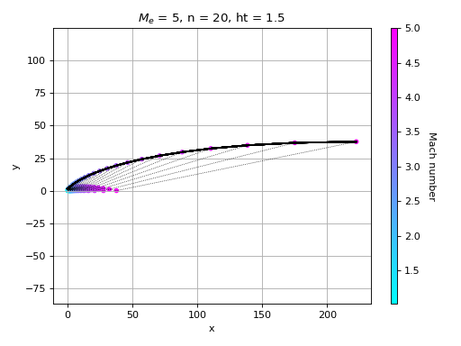
from pygasflow.nozzles.moc import min_length_supersonic_nozzle_moc
import numpy as np
import matplotlib.pyplot as plt
import matplotlib.cm as cmx
ht = 1.5
n = 20
Me = 5
gamma = 1.4
wall, characteristics, left_runn_chars, theta_w_max = min_length_supersonic_nozzle_moc(ht, n, Me, None, gamma)
x, y, z = np.array([]), np.array([]), np.array([])
for char in left_runn_chars:
    x = np.append(x, char["x"])
    y = np.append(y, char["y"])
    z = np.append(z, char["M"])
plt.figure()
# draw characteristics lines
for c in characteristics:
    plt.plot(c["x"], c["y"], "k:", linewidth=0.65)
    # draw nozzle wall
    plt.plot(wall[:, 0], wall[:, 1], "k")
# over impose grid points colored by Mach number
sc = plt.scatter(x, y, c=z, s=15, vmin=min(z), vmax=max(z), cmap=cmx.cool)
cbar = plt.colorbar(sc, orientation='vertical', aspect=40)
cbar.ax.get_yaxis().labelpad = 15
cbar.ax.set_ylabel("Mach number", rotation=270)
plt.xlabel("x")
plt.ylabel("y")
plt.title(r"$M_e$ = {}, n = {}, ht = {} ".format(Me, n, ht))
plt.grid()
plt.axis('equal')
plt.tight_layout()
plt.show()
(
Source code,png,hires.png,pdf)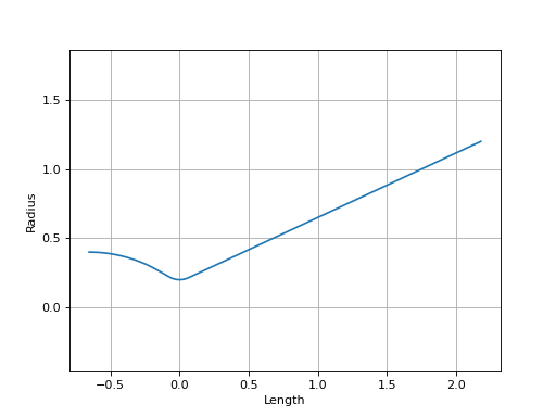
- class pygasflow.nozzles.moc.CD_Min_Length_Nozzle(Ri=0.4, Re=1.2, Rt=0.2, Rj=0.1, R0=0, theta_c=40, n_lines=10, gamma=1.4, **params)[source]
Planar Convergent-Divergent nozzle based on Minimum Length computed with the Method of Characteristics.
- Parameters:
- inlet_radiusNumber
- bounds:
inlet_radius >= 0
- default:
0.4
Alias
Riin the constructor.- outlet_radiusNumber
- bounds:
outlet_radius >= 0
- default:
1.2
Alias
Rein the constructor.- throat_radiusNumber
- bounds:
throat_radius >= 0
- default:
0.2
Alias
Rtin the constructor.- theta_cNumber
- bounds:
\(0 < \theta_{c} < 90\)
- default:
40
Half angle [degrees] of the convergent
- NInteger
- bounds:
10 <= N <= 1000
- default:
200
Number of discretization elements along the length of the nozzle.
- gammaNumber
- bounds:
1 < gamma <= 2
- default:
1.4
Ratio of specific heats, γ = Cp / Cv
- n_linesInteger
- bounds:
n_lines >= 3
- default:
10
- inlet_areaNumber
- bounds:
inlet_area >= 0
- read only:
True
- outlet_areaNumber
- bounds:
outlet_area >= 0
- read only:
True
- throat_areaNumber
- bounds:
throat_area >= 0
- read only:
True
- length_convergentNumber
- allow_None:
True
- default:
0.0
- length_divergentNumber
- allow_None:
True
- default:
0.0
- lengthNumber
- bounds:
length >= 0
- default:
0.0
Total length of the nozzle, convergent + divergent.
- shockwave_locationTuple
- constant:
True
- default:
(None, None)
- length:
2
Location of the shockwave in the divergent: (loc, radius).
- theta_w_maxNumber
- read only:
True
Maximum angle of the wall.
- wallArray
- allow_None:
True
- constant:
True
Mx2 array of wall coordinates computed by MOC. First column is the x-coordinates, second column is the y-coordinates.
- characteristicsList
- constant:
True
- default:
[]
- item_type:
dict
List of dictionaries. Each dictionary contains the keys “x”, “y” for the coordinates of the points of each characteristic. Here, with characteristic, I mean the points of the right and left running characteristic.
- left_runn_charsList
- constant:
True
- default:
[]
- item_type:
dict
List of dictionaries. Each dictionary contains the keys “Km”, “Kp”, “theta”, “nu”, “M”, “mu”, “x”, “y”. Each dictionary represents the points lying on the same left-running characteristic.
Examples
Compute the length of a minimum length nozzle:
>>> from pygasflow.nozzles import CD_Conical_Nozzle
>>> Ri, Re, Rt = 0.4, 1.2, 0.2
>>> nozzle = CD_Conical_Nozzle(Ri, Re, Rt, theta_c=30, theta_N=25)
>>> nozzle.length
np.float64(2.53988146753074)
Change the angle of the divergent section and retrieve the new length of the nozzle:
>>> nozzle.theta_N = 60
>>> nozzle.length
np.float64(1.0082903768654763)
Visualize the nozzle:
from pygasflow.nozzles import CD_Min_Length_Nozzle
Ri, Re, Rt = 0.4, 0.5, 0.2
nozzle = CD_Min_Length_Nozzle(Ri, Re, Rt, theta_c=30, n_lines=20)
nozzle.plot(interactive=False, show_characteristic_lines=True)
- pygasflow.nozzles.moc.CD_Min_Length_Nozzle.get_points(self, area_ratio=False, offset=1.2)
Helper function used to construct a matrix of points representing the nozzle for visualization purposes.
- Parameters:
- area_ratioBoolean
If True, represents the area ratio \(\frac{A}{A^{*}}\). Otherwise, represents the radius. Default to False.
- offsetfloat
Used to construct the container (or the walls) of the nozzle. The container radius is equal to offset * max_nozzle_radius.
- Returns:
- flow_areanp.ndarray [Nx2]
Matrix representing the flow area.
- containernp.ndarray [Nx2]
Matrix representing the outer walls of the nozzle.
- pygasflow.nozzles.moc.CD_Min_Length_Nozzle.location_divergent_from_area_ratio(self, A_ratio)
Given an area ratio, compute the location on the divergent where this area ratio is located.
- Parameters:
- A_ratiofloat
A / At
- Returns:
- xfloat or None
x-coordinate along the divergent length. If A_ratio > Ae / At, it returns None.
- pygasflow.nozzles.moc.CD_Min_Length_Nozzle.plot(self, interactive=True, **kwargs)
- Parameters:
- interactivebool
If False, shows and return a Bokeh figure. If True, returns a servable object, which will be automatically rendered inside a Jupyter Notebook. If any other interpreter is used, then
nozzle.plot(interactive=True).show()might be required in order to visualize the interactive application.
Rao Parabola Angles
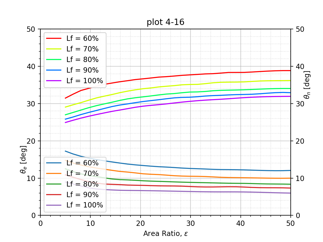
- class pygasflow.nozzles.rao_parabola_angles.Rao_Parabola_Angles[source]
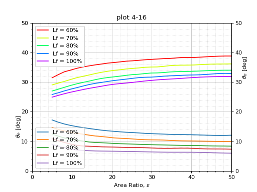
This class is used to generate the relation from the extracted data of plot 4-16, page 77, Modern Engineering for Design of Liquid-Propellant Rocket Engines, D.K. Huzel and D.H. Huang.
Useful for finding the Rao’s parabola angles given the fractional length and the area ratio, or vice-versa.
The plot relate the Rao’s TOP nozzle:
theta_n, initial parabola angle
theta_e, final parabola angle
with the expansion ratio, epsilon, varying the fractional nozzle length Lf.
Note that the data has been manually extracted from the plot in the book, hence it is definitely a huge “approximation”. If you have the original Rao’s plot, you can probably extract better data.
Examples
Visualize the plot:
from pygasflow import Rao_Parabola_Angles
p = Rao_Parabola_Angles()
p.plot()
(
Source code,png,hires.png,pdf)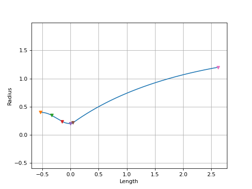
Compute the angles at the end points of Rao’s parabola for a nozzle with fractional length 68 and area ratio 35:
>>> from pygasflow import Rao_Parabola_Angles
>>> p = Rao_Parabola_Angles()
>>> print(p.angles_from_Lf_Ar(68, 35))
(np.float64(36.11883335948745), np.float64(10.695233384809715))
Compute the area ratio for a nozzle with fractional length 68 and an angle at the start of the parabola of 35 degrees:
>>> p.area_ratio_from_Lf_angle(68, theta_n=35)
np.float64(24.83022334667575)
- pygasflow.nozzles.rao_parabola_angles.Rao_Parabola_Angles.angles_from_Lf_Ar(self, Lf, Ar)
Compute the angles at the end points of Rao’s parabola. Note that linear interpolation is used if Lf is different than 60, 70, 80, 90, 100.
- Parameters:
- Lffloat
Fractional length in percent. Must be 60 <= Lf <= 100.
- Arfloat
Area ratio. Must be 5 <= Ar <= 50.
- Returns:
- theta_nfloat
Angle in degrees at the start of the parabola.
- theta_efloat
Angle in degrees at the end of the parabola (at the exit section).
- pygasflow.nozzles.rao_parabola_angles.Rao_Parabola_Angles.area_ratio_from_Lf_angle(self, Lf=60, **kwargs)
Compute the Area Ratio given Lf, theta_n or theta_e.
- Parameters:
- Lffloat
Fractional length in percent. Must be 60 <= Lf <= 100.
- kwargsfloat.
It can either be:
- theta_nfloat
The angle in degrees at the start of the parabola.
- theta_efloat
The angle in degrees at the end of the parabola.
- Returns:
- Arfloat
The area ratio corresponding to the given angle and Lf. Note that linear interpolation is used if Lf is different than 60, 70, 80, 90, 100.
- pygasflow.nozzles.rao_parabola_angles.Rao_Parabola_Angles.plot(self, N=30)
Plot the relation.
- Parameters:
- Nint
Number of interpolated point for each curve. Default to 30.