Solvers
All the following solvers accepts the to_dict keyword argument:
to_dict=False: returns a list of results.to_dict=True: returns a dictionary of results. This option has a few advantages:it is easier to retrieve a particular quantity from a dictionary of results, because user only needs to remember the key name, which are often self explanatory, for example
"pr"stands for pressure ratio. On the other hand, with a list of results user needs to remember the index of a particular quantity.it is easier to maintain back-compatibility. Suppose users are returning list of results from a solver, and accessing a particular quantity with some index. Time passes and the module gets implemented further, maybe new quantities are added to the list of results, maybe some quantity is removed. At this point, user’s code may be broken. This is unlikely to happen with a dictionary of results, where deprecation warning can easily be inserted when a particular key is accessed, informing users on the best course of action.
The default behavior is to_dict=False (for back-compatibility reasons).
If we are executing multiple solver calls and we are interested in
dictionaries of results, the quickest way is by setting a global
default option of the module, thus skipping the to_dict keyword argument:
Regardless of the to_dict option, results returned from the solvers are
enhanced lists/dicts, which exposes the show() method in order to
print a nice tables with numerical results and explanatory labels.
Here is an example. As we load the module, the solver returns a list of results:
>>> import pygasflow
>>> from pygasflow.solvers import (
...     isentropic_solver,
...     oblique_shockwave_solver,
...     fanno_solver,
... )
>>> res_ise = isentropic_solver("m", 3)
>>> isinstance(res_ise, list)
True
>>> res_ise
[np.float64(3.0), np.float64(0.02722368370386282), np.float64(0.0762263143708159), np.float64(0.35714285714285715), np.float64(0.051532504691298484), np.float64(0.12024251094636311), np.float64(0.4285714285714286), np.float64(1.9639610121239315), np.float64(4.234567901234571), np.float64(19.47122063449069), np.float64(49.75734674434607)]
>>> res_ise.show()
idx   quantity
--------------------------
0     M                        3.00000000
1     P / P0                   0.02722368
2     rho / rho0               0.07622631
3     T / T0                   0.35714286
4     P / P*                   0.05153250
5     rho / rho*               0.12024251
6     T / T*                   0.42857143
7     U / U*                   1.96396101
8     A / A*                   4.23456790
9     Mach Angle              19.47122063
10    Prandtl-Meyer           49.75734674
We can change the global option, after which all solvers will return dictionaries of results:
>>> pygasflow.defaults.solver_to_dict = True
>>> res_ise = isentropic_solver("m", 3)
>>> isinstance(res_ise, dict)
True
>>> res_ise
{'m': np.float64(3.0), 'pr': np.float64(0.02722368370386282), 'dr': np.float64(0.0762263143708159), 'tr': np.float64(0.35714285714285715), 'prs': np.float64(0.051532504691298484), 'drs': np.float64(0.12024251094636311), 'trs': np.float64(0.4285714285714286), 'urs': np.float64(1.9639610121239315), 'ars': np.float64(4.234567901234571), 'ma': np.float64(19.47122063449069), 'pm': np.float64(49.75734674434607)}
>>> res_ise.show()
key     quantity
----------------------------
m       M                        3.00000000
pr      P / P0                   0.02722368
dr      rho / rho0               0.07622631
tr      T / T0                   0.35714286
prs     P / P*                   0.05153250
drs     rho / rho*               0.12024251
trs     T / T*                   0.42857143
urs     U / U*                   1.96396101
ars     A / A*                   4.23456790
ma      Mach Angle              19.47122063
pm      Prandtl-Meyer           49.75734674
>>> res_shock = oblique_shockwave_solver("mu", 4, "theta", 15, flag="weak")
>>> isinstance(res_shock, dict)
True
>>> res_shock
{'mu': np.float64(4.0), 'mnu': np.float64(1.819872100323947), 'md': np.float64(2.929007710626549), 'mnd': np.float64(0.6121186581027711), 'beta': np.float64(27.062876925385396), 'theta': np.float64(15.0), 'pr': np.float64(3.6972568717937433), 'dr': np.float64(2.3907318881276685), 'tr': np.float64(1.546495820026601), 'tpr': np.float64(0.803820352213437)}
>>> res_shock.show()
key     quantity
---------------------
mu      Mu                4.00000000
mnu     Mnu               1.81987210
md      Md                2.92900771
mnd     Mnd               0.61211866
beta    beta             27.06287693
theta   theta            15.00000000
pr      pd/pu             3.69725687
dr      rhod/rhou         2.39073189
tr      Td/Tu             1.54649582
tpr     p0d/p0u           0.80382035
It must be noted that we can still force a solver to return a list of results
by setting the to_dict = False keyword argument. In other words, this
keyword argument has a stronger priority than the global option:
>>> res_ise = isentropic_solver("m", 3, to_dict=False)
>>> isinstance(res_ise, list)
True
Now, to go back to the default behavior, which returns list of results:
>>> pygasflow.defaults.solver_to_dict = False
>>> res_fanno = fanno_solver("m", 4)
>>> isinstance(res_fanno, list)
True
>>> res_fanno
[np.float64(4.0), np.float64(0.1336306209562122), np.float64(0.46770717334674267), np.float64(0.28571428571428575), np.float64(10.718750000000002), np.float64(2.138089935299395), np.float64(0.6330649317809258), np.float64(2.3719945443662134)]
Isentropic Solver
- pygasflow.solvers.isentropic.isentropic_solver(param_name, param_value, gamma=1.4, to_dict=None)[source]
Compute all isentropic ratios and Mach number given an input parameter.
- Parameters:
- param_namestring
Name of the parameter given in input. Can be either one of:
'm': Mach number'pressure': Pressure Ratio \(\frac{P}{P_{0}}\)'density': Density Ratio \(\frac{\rho}{\rho_{0}}\)'temperature': Temperature Ratio \(\frac{T}{T_{0}}\)'crit_area_sub': Critical Area Ratio \(\frac{A}{A^{*}}\) for subsonic case.'crit_area_super': Critical Area Ratio \(\frac{A}{A^{*}}\) for supersonic case.'mach_angle': Mach Angle in degrees.'prandtl_meyer': Prandtl-Meyer Angle in degrees.
- param_valuefloat/list/array_like
Actual value of the parameter. If float, list, tuple is given as input, a conversion will be attempted.
- gammafloat, optional
Specific heats ratio. Default to 1.4. Must be > 1.
- to_dictbool, optional
If False, the function returns a list of results. If True, it returns a dictionary in which the keys are listed in the Returns section. Default to False (return a list of results).
- Returns:
- marray_like
Mach number
- prarray_like
Pressure Ratio \(\frac{P}{P_{0}}\)
- drarray_like
Density Ratio \(\frac{\rho}{\rho_{0}}\)
- trarray_like
Temperature Ratio \(\frac{T}{T_{0}}\)
- prsarray_like
Critical Pressure Ratio \(\frac{P}{P^{*}}\)
- drsarray_like
Critical Density Ratio \(\frac{\rho}{\rho^{*}}\)
- trsarray_like
Critical Temperature Ratio \(\frac{T}{T^{*}}\)
- ursarray_like
Critical Velocity Ratio \(\frac{U}{U^{*}}\)
- arsarray_like
Critical Area Ratio \(\frac{A}{A^{*}}\)
- maarray_like
Mach Angle
- pmarray_like
Prandtl-Meyer Angle
Examples
Compute all ratios starting from a single Mach number:
>>> from pygasflow.solvers import isentropic_solver
>>> res = isentropic_solver("m", 2)
>>> res
[np.float64(2.0), np.float64(0.12780452546295096), np.float64(0.23004814583331168), np.float64(0.5555555555555556), np.float64(0.24192491286747442), np.float64(0.36288736930121157), np.float64(0.6666666666666667), np.float64(1.632993161855452), np.float64(1.6875000000000002), np.float64(30.000000000000004), np.float64(26.379760813416457)]
>>> res.show()
idx   quantity
--------------------------
0     M                        2.00000000
1     P / P0                   0.12780453
2     rho / rho0               0.23004815
3     T / T0                   0.55555556
4     P / P*                   0.24192491
5     rho / rho*               0.36288737
6     T / T*                   0.66666667
7     U / U*                   1.63299316
8     A / A*                   1.68750000
9     Mach Angle              30.00000000
10    Prandtl-Meyer           26.37976081
Compute all parameters starting from the pressure ratio:
>>> res = isentropic_solver("pressure", 0.12780452546295096)
>>> res.show()
idx   quantity
--------------------------
0     M                        2.00000000
1     P / P0                   0.12780453
2     rho / rho0               0.23004815
3     T / T0                   0.55555556
4     P / P*                   0.24192491
5     rho / rho*               0.36288737
6     T / T*                   0.66666667
7     U / U*                   1.63299316
8     A / A*                   1.68750000
9     Mach Angle              30.00000000
10    Prandtl-Meyer           26.37976081
Compute the Mach number starting from the Mach Angle:
>>> results = isentropic_solver("mach_angle", 25)
>>> results.show()
idx   quantity
--------------------------
0     M                        2.36620158
1     P / P0                   0.07210756
2     rho / rho0               0.15285231
3     T / T0                   0.47174663
4     P / P*                   0.13649451
5     rho / rho*               0.24111550
6     T / T*                   0.56609595
7     U / U*                   1.78031465
8     A / A*                   2.32958260
9     Mach Angle              25.00000000
10    Prandtl-Meyer           35.92354277
>>> print(results[0])
2.3662015831524985
Compute the pressure ratios starting from two Mach numbers:
>>> results = isentropic_solver("m", [2, 3])
>>> results.show()
idx   quantity
--------------------------
0     M                        2.00000000     3.00000000
1     P / P0                   0.12780453     0.02722368
2     rho / rho0               0.23004815     0.07622631
3     T / T0                   0.55555556     0.35714286
4     P / P*                   0.24192491     0.05153250
5     rho / rho*               0.36288737     0.12024251
6     T / T*                   0.66666667     0.42857143
7     U / U*                   1.63299316     1.96396101
8     A / A*                   1.68750000     4.23456790
9     Mach Angle              30.00000000    19.47122063
10    Prandtl-Meyer           26.37976081    49.75734674
>>> print(results[1])
[0.12780453 0.02722368]
Compute the pressure ratios starting from two Mach numbers, returning a dictionary:
>>> results = isentropic_solver("m", [2, 3], to_dict=True)
>>> results.show()
key     quantity
----------------------------
m       M                        2.00000000     3.00000000
pr      P / P0                   0.12780453     0.02722368
dr      rho / rho0               0.23004815     0.07622631
tr      T / T0                   0.55555556     0.35714286
prs     P / P*                   0.24192491     0.05153250
drs     rho / rho*               0.36288737     0.12024251
trs     T / T*                   0.66666667     0.42857143
urs     U / U*                   1.63299316     1.96396101
ars     A / A*                   1.68750000     4.23456790
ma      Mach Angle              30.00000000    19.47122063
pm      Prandtl-Meyer           26.37976081    49.75734674
>>> print(results["pr"])
[0.12780453 0.02722368]
- pygasflow.solvers.isentropic.print_isentropic_results(results, number_formatter=None, blank_line=False)[source]
- Parameters:
- resultslist or dict
- number_formatterstr or None
A formatter to properly show floating point numbers. For example,
"{:>8.3f}"to show numbers with 3 decimal places.- blank_linebool
If True, a blank line will be printed after the results.
See also
- pygasflow.solvers.isentropic.isentropic_compression(pr=None, dr=None, tr=None, gamma=1.4, to_dict=None)[source]
Solve the isentropic compression (or expansion) by providing a ratio.
- Parameters:
- prarray_like, optional
Pressure ratio p2/p1
- drarray_like, optional
Density ratio rho2/rho1
- trarray_like, optional
Temperature ratio T2/T1
- gammafloat, optional
Specific heats ratio. Must be \(\gamma > 1\).
- to_dictbool, optional
If False, the function returns a list of results. If True, it returns a dictionary in which the keys are listed in the Returns section. Default to False (return a list of results).
- Returns:
- prarray_like
Pressure ratio p2/p1
- drarray_like
Density ratio rho2/rho1
- trarray_like
Temperature ratio T2/T1
See also
Examples
>>> from pygasflow import isentropic_compression
>>> T1 = 290    # K
>>> res = isentropic_compression(pr=2, to_dict=True)
>>> res.show()
key     quantity
----------------------------
pr      P2 / P1                  2.00000000
dr      rho2 / rho1              1.64067071
tr      T2 / T1                  1.21901365
>>> T2_T1 = res["tr"]
>>> T2 = T2_T1 * T1
>>> T2
np.float64(353.5139597192979)
Fanno Solver
- pygasflow.solvers.fanno.fanno_solver(param_name, param_value, gamma=1.4, to_dict=None)[source]
Given an input parameter, compute all ratios and Mach number of a 1-D flow with friction (Fanno flow).
- Parameters:
- param_namestring
Name of the parameter given in input. Can be either one of:
'm': Mach number'pressure': Critical Pressure Ratio \(\frac{P}{P^{*}}\)'density': Critical Density Ratio \(\frac{\rho}{\rho^{*}}\)'temperature': Critical Temperature Ratio \(\frac{T}{T^{*}}\)'total_pressure_sub': Critical Total Pressure Ratio \(\frac{P_{0}}{P_{0}^{*}}\) for subsonic case.'total_pressure_super': Critical Total Pressure Ratio \(\frac{P_{0}}{P_{0}^{*}}\) for supersonic case.'velocity': Critical Velocity Ratio \(\frac{U}{U^{*}}\).'friction_sub': Critical Friction parameter \(\frac{4 f L^{*}}{D}\) for subsonic case.'friction_super': Critical Friction parameter \(\frac{4 f L^{*}}{D}\) for supersonic case.'entropy_sub': Entropy parameter \(\frac{s^{*} - s}{R}\) for subsonic case.'entropy_super': Entropy parameter \(\frac{s^{*} - s}{R}\) for supersonic case.
- param_valuefloat/list/array_like
Actual value of the parameter. If float, list, tuple is given as input, a conversion will be attempted.
- gammafloat, optional
Specific heats ratio. Default to 1.4. Must be > 1.
- to_dictbool, optional
If False, the function returns a list of results. If True, it returns a dictionary in which the keys are listed in the Returns section. Default to False (return a list of results).
- Returns:
- marray_like
Mach number
- prsarray_like
Critical Pressure Ratio \(\frac{P}{P^{*}}\)
- drsarray_like
Critical Density Ratio \(\frac{\rho}{\rho^{*}}\)
- trsarray_like
Critical Temperature Ratio \(\frac{T}{T^{*}}\)
- tprsarray_like
Critical Total Pressure Ratio \(\frac{P_{0}}{P_{0}^{*}}\)
- ursarray_like
Critical Velocity Ratio \(\frac{U}{U^{*}}\)
- fpsarray_like
Critical Friction Parameter \(\frac{4 f L^{*}}{D}\)
- epsarray_like
Critical Entropy Ratio \(\frac{s^{*} - s}{R}\)
See also
Examples
Compute all ratios starting from a Mach number:
>>> from pygasflow.solvers import fanno_solver
>>> res = fanno_solver("m", 2)
>>> res
[np.float64(2.0), np.float64(0.408248290463863), np.float64(0.6123724356957945), np.float64(0.6666666666666667), np.float64(1.6875000000000002), np.float64(1.632993161855452), np.float64(0.3049965025814798), np.float64(0.523248143764548)]
>>> res.show()
idx   quantity
-------------------
0     M                 2.00000000
1     P / P*            0.40824829
2     rho / rho*        0.61237244
3     T / T*            0.66666667
4     P0 / P0*          1.68750000
5     U / U*            1.63299316
6     4fL* / D          0.30499650
7     (s*-s) / R        0.52324814
Compute the subsonic Mach number starting from the critical friction parameter:
>>> results = fanno_solver("friction_sub", 0.3049965025814798)
>>> results.show()
idx   quantity
-------------------
0     M                 0.65725799
1     P / P*            1.59904374
2     rho / rho*        1.44766442
3     T / T*            1.10456796
4     P0 / P0*          1.12898142
5     U / U*            0.69076782
6     4fL* / D          0.30499650
7     (s*-s) / R        0.12131583
>>> print(results[0])
0.6572579935727846
Compute the critical temperature ratio starting from multiple Mach numbers for a gas having specific heat ratio gamma=1.2:
>>> results = fanno_solver("m", [0.5, 1.5], 1.2)
>>> results.show()
idx   quantity
-------------------
0     M                 0.50000000     1.50000000
1     P / P*            2.07187908     0.63173806
2     rho / rho*        1.93061460     0.70352647
3     T / T*            1.07317073     0.89795918
4     P0 / P0*          1.35628665     1.20502889
5     U / U*            0.51796977     1.42141062
6     4fL* / D          1.29396294     0.18172829
7     (s*-s) / R        0.30475056     0.18650354
>>> print(results[3])
[1.07317073 0.89795918]
Compute the critical temperature ratio starting from multiple Mach numbers for a gas having specific heat ratio gamma=1.2, returning a dictionary:
>>> results = fanno_solver("m", [0.5, 1.5], 1.2, to_dict=True)
>>> results
{'m': array([0.5, 1.5]), 'prs': array([2.07187908, 0.63173806]), 'drs': array([1.9306146 , 0.70352647]), 'trs': array([1.07317073, 0.89795918]), 'tprs': array([1.35628665, 1.20502889]), 'urs': array([0.51796977, 1.42141062]), 'fps': array([1.29396294, 0.18172829]), 'eps': array([0.30475056, 0.18650354])}
>>> results.show()
key     quantity
---------------------
m       M                 0.50000000     1.50000000
prs     P / P*            2.07187908     0.63173806
drs     rho / rho*        1.93061460     0.70352647
trs     T / T*            1.07317073     0.89795918
tprs    P0 / P0*          1.35628665     1.20502889
urs     U / U*            0.51796977     1.42141062
fps     4fL* / D          1.29396294     0.18172829
eps     (s*-s) / R        0.30475056     0.18650354
>>> print(results["trs"])
[1.07317073 0.89795918]
- pygasflow.solvers.fanno.print_fanno_results(results, number_formatter=None, blank_line=False)[source]
- Parameters:
- resultslist or dict
- number_formatterstr or None
A formatter to properly show floating point numbers. For example,
"{:>8.3f}"to show numbers with 3 decimal places.- blank_linebool
If True, a blank line will be printed after the results.
See also
Rayleigh Solver
- pygasflow.solvers.rayleigh.rayleigh_solver(param_name, param_value, gamma=1.4, to_dict=None)[source]
Given an input parameter, compute all ratios and Mach number of 1-D flow with heat addition (Rayleigh flow).
- Parameters:
- param_namestring
Name of the parameter given in input. Can be either one of:
'm': Mach number'pressure': Critical Pressure Ratio \(\frac{P}{P^{*}}\)'density': Critical Density Ratio \(\frac{\rho}{\rho^{*}}\)'velocity': Critical Velocity Ratio \(\frac{U}{U^{*}}\).'temperature_sub': Critical Temperature Ratio \(\frac{T}{T^{*}}\) for subsonic case.'temperature_super': Critical Temperature Ratio \(\frac{T}{T^{*}}\) for supersonic case.'total_pressure_sub': Critical Total Pressure Ratio \(\frac{P_{0}}{P_{0}^{*}}\) for subsonic case.'total_pressure_super': Critical Total Pressure Ratio \(\frac{P_{0}}{P_{0}^{*}}\) for supersonic case.'total_temperature_sub': Critical Total Temperature Ratio \(\frac{T_{0}}{T_{0}^{*}}\) for subsonic case.'total_temperature_super': Critical Total Temperature Ratio \(\frac{T_{0}}{T_{0}^{*}}\) for supersonic case.'entropy_sub': Entropy parameter \(\frac{s^{*} - s}{R}\) for subsonic case.'entropy_super': Entropy parameter \(\frac{s^{*} - s}{R}\) for supersonic case.
- param_valuefloat/list/array_like
Actual value of the parameter. If float, list, tuple is given as input, a conversion will be attempted.
- gammafloat, optional
Specific heats ratio. Default to 1.4. Must be > 1.
- to_dictbool, optional
If False, the function returns a list of results. If True, it returns a dictionary in which the keys are listed in the Returns section. Default to False (return a list of results).
- Returns:
- marray_like
Mach number
- prsarray_like
Critical Pressure Ratio \(\frac{P}{P^{*}}\)
- drsarray_like
Critical Density Ratio \(\frac{\rho}{\rho^{*}}\)
- trsarray_like
Critical Temperature Ratio \(\frac{T}{T^{*}}\)
- tprsarray_like
Critical Total Pressure Ratio \(\frac{P_{0}}{P_{0}^{*}}\)
- ttrsarray_like
Critical Total Temperature Ratio \(\frac{T_{0}}{T_{0}^{*}}\)
- ursarray_like
Critical Velocity Ratio \(\frac{U}{U^{*}}\)
- epsarray_like
Critical Entropy Ratio \(\frac{s^{*} - s}{R}\)
See also
Examples
Compute all ratios starting from a single Mach number:
>>> from pygasflow.solvers import rayleigh_solver
>>> res = rayleigh_solver("m", 2)
>>> res
[np.float64(2.0), np.float64(0.36363636363636365), np.float64(0.6875), np.float64(0.5289256198347108), np.float64(1.5030959785260414), np.float64(0.793388429752066), np.float64(1.4545454545454546), np.float64(1.2175752061512626)]
>>> res.show()
idx   quantity
-------------------
0     M                 2.00000000
1     P / P*            0.36363636
2     rho / rho*        0.68750000
3     T / T*            0.52892562
4     P0 / P0*          1.50309598
5     T0 / T0*          0.79338843
6     U / U*            1.45454545
7     (s*-s) / R        1.21757521
Compute the subsonic Mach number starting from the critical entropy ratio:
>>> res = rayleigh_solver("entropy_sub", 0.5)
>>> res.show()
idx   quantity
-------------------
0     M                 0.66341885
1     P / P*            1.48498826
2     rho / rho*        1.53003501
3     T / T*            0.97055835
4     P0 / P0*          1.05396114
5     T0 / T0*          0.87999306
6     U / U*            0.65357982
7     (s*-s) / R        0.50000000
>>> print(res[0])
0.6634188478510624
Compute the critical temperature ratio starting from multiple Mach numbers for a gas having specific heat ratio gamma=1.2:
>>> res = rayleigh_solver("m", [0.5, 1.5], 1.2)
>>> res.show()
idx   quantity
-------------------
0     M                 0.50000000     1.50000000
1     P / P*            1.69230769     0.59459459
2     rho / rho*        2.36363636     0.74747475
3     T / T*            0.71597633     0.79547115
4     P0 / P0*          1.10781288     1.13417842
5     T0 / T0*          0.66715976     0.88586560
6     U / U*            0.42307692     1.33783784
7     (s*-s) / R        2.53074211     0.85304875
>>> print(res[3])
[0.71597633 0.79547115]
Compute the critical temperature ratio starting from multiple Mach numbers for a gas having specific heat ratio gamma=1.2, returning a dictionary:
>>> res = rayleigh_solver("m", [0.5, 1.5], 1.2, to_dict=True)
>>> res.show()
key     quantity
---------------------
m       M                 0.50000000     1.50000000
prs     P / P*            1.69230769     0.59459459
drs     rho / rho*        2.36363636     0.74747475
trs     T / T*            0.71597633     0.79547115
tprs    P0 / P0*          1.10781288     1.13417842
ttrs    T0 / T0*          0.66715976     0.88586560
urs     U / U*            0.42307692     1.33783784
eps     (s*-s) / R        2.53074211     0.85304875
>>> print(res["trs"])
[0.71597633 0.79547115]
- pygasflow.solvers.rayleigh.print_rayleigh_results(results, number_formatter=None, blank_line=False)[source]
- Parameters:
- resultslist or dict
- number_formatterstr or None
A formatter to properly show floating point numbers. For example,
"{:>8.3f}"to show numbers with 3 decimal places.- blank_linebool
If True, a blank line will be printed after the results.
See also
Shockwave Solvers
- pygasflow.solvers.shockwave.normal_shockwave_solver(param_name, param_value, gamma=1.4, to_dict=None)[source]
Compute all the ratios across a normal shock wave.
- Parameters:
- param_namestring
Name of the parameter given in input. In the following ratios, d stands for downstream of the shockwave while u stand for upstream of the shockwave. Can be either one of:
'pressure': Pressure Ratio \(\frac{P_{d}}{P_{u}}\)'temperature': Temperature Ratio \(\frac{T_{d}}{T_{u}}\)'density': Density Ratio \(\frac{\rho_{d}}{\rho_{u}}\)'total_pressure': Total Pressure Ratio \(\frac{P_{d}^{0}}{P_{u}^{0}}\)'mu': upstream Mach number of the shock wave'md': downstream Mach number of the shock wave
If the parameter is a ratio, it is in the form downstream/upstream.
- param_valuefloat
Actual value of the parameter.
- gammafloat, optional
Specific heats ratio. Default to 1.4. Must be > 1.
- to_dictbool, optional
If False, the function returns a list of results. If True, it returns a dictionary in which the keys are listed in the Returns section. Default to False (return a list of results).
- Returns:
- mufloat
Mach number upstream of the shock wave.
- mdfloat
Mach number downstream of the shock wave.
- prfloat
Pressure ratio across the shock wave.
- drfloat
Density ratio across the shock wave.
- trfloat
Temperature ratio across the shock wave.
- tprfloat
Total Pressure ratio across the shock wave.
Examples
Compute all ratios across a normal shockwave starting with the upstream Mach number, using air:
>>> from pygasflow.solvers import normal_shockwave_solver
>>> res = normal_shockwave_solver("mu", 2)
>>> isinstance(res, list)
True
>>> res.show()
idx   quantity
-------------------
0     Mu                2.00000000
1     Md                0.57735027
2     pd/pu             4.50000000
3     rhod/rhou         2.66666667
4     Td/Tu             1.68750000
5     p0d/p0u           0.72087386
Compute all ratios and parameters across a normal shockwave starting from the downstream Mach number, using methane at 20°C:
>>> res = normal_shockwave_solver("md", 0.4, gamma=1.32)
>>> res.show()
idx   quantity
-------------------
0     Mu                4.47562845
1     Md                0.40000000
2     pd/pu            22.65625000
3     rhod/rhou         5.52586207
4     Td/Tu             4.10003900
5     p0d/p0u           0.06721057
Compute the Mach number downstream of an oblique shockwave starting with multiple upstream Mach numbers, returning a dictionary:
>>> res = normal_shockwave_solver("mu", [1.5, 3], to_dict=True)
>>> isinstance(res, dict)
True
>>> res.show()
key     quantity
---------------------
mu      Mu                1.50000000     3.00000000
md      Md                0.70108874     0.47519096
pr      pd/pu             2.45833333    10.33333333
dr      rhod/rhou         1.86206897     3.85714286
tr      Td/Tu             1.32021605     2.67901235
tpr     p0d/p0u           0.92978651     0.32834389
>>> print(res["md"])
[0.70108874 0.47519096]
- pygasflow.solvers.shockwave.print_normal_shockwave_results(results, number_formatter=None, blank_line=False)[source]
- Parameters:
- resultslist or dict
- number_formatterstr or None
A formatter to properly show floating point numbers. For example,
"{:>8.3f}"to show numbers with 3 decimal places.- blank_linebool
If True, a blank line will be printed after the results.
See also
- pygasflow.solvers.shockwave.oblique_shockwave_solver(p1_name, p1_value, p2_name='beta', p2_value=90, gamma=1.4, flag='weak', to_dict=None)[source]
Attempt to compute all the ratios, angles and mach numbers across the shock wave.
An alias of this function is shockwave_solver.
- Parameters:
- p1_namestring
Name of the first parameter given in input. In the following ratios, d stands for downstream of the shockwave while u stand for upstream of the shockwave. Can be either one of:
'pressure': Pressure Ratio \(\frac{P_{d}}{P_{u}}\)'temperature': Temperature Ratio \(\frac{T_{d}}{T_{u}}\)'density': Density Ratio \(\frac{\rho_{d}}{\rho_{u}}\)'total_pressure': Total Pressure Ratio \(\frac{P_{d}^{0}}{P_{u}^{0}}\)'mu': upstream Mach number of the shock wave'mnu': upstream normal Mach number of the shock wave'mnd': downstream normal Mach number of the shock wave'beta': The shock wave angle [in degrees]. It can only be used ifp2_name='theta'.'theta': The deflection angle [in degrees]. It can only be used ifp2_name='beta'.
If the parameter is a ratio, it is in the form downstream/upstream.
- p1_valuefloat
Actual value of the parameter.
- p2_namestring, optional
Name of the second parameter. It could either be:
'beta': Shock wave angle.'theta': Flow deflection angle.'mnu': upstream normal Mach number.
Default to
'beta'.- p2_valuefloat, optional
Value of the angle in degrees. Default to 90 degrees (normal shock wave).
- gammafloat, optional
Specific heats ratio. Default to 1.4. Must be > 1.
- flagstring, optional
Chose what solution to compute if the angle ‘theta’ is provided. Can be either
'weak'or'strong'. Default to'weak'.- to_dictbool, optional
If False, the function returns a list of results. If True, it returns a dictionary in which the keys are listed in the Returns section. Default to False (return a list of results).
- Returns:
- mufloat
Mach number upstream of the shock wave.
- mnufloat
Normal Mach number upstream of the shock wave.
- mdfloat
Mach number downstream of the shock wave.
- mndfloat
Normal Mach number downstream of the shock wave.
- betafloat
Shock wave angle in degrees.
- thetafloat
Flow deflection angle in degrees.
- prfloat
Pressure ratio across the shock wave.
- drfloat
Density ratio across the shock wave.
- trfloat
Temperature ratio across the shock wave.
- tprfloat
Total Pressure ratio across the shock wave.
Examples
Compute all ratios across a weak oblique shockwave starting with the upstream Mach number and the deflection angle, using air:
>>> from pygasflow.solvers import oblique_shockwave_solver
>>> res = oblique_shockwave_solver("mu", 2, "theta", 15, flag="weak")
>>> isinstance(res, list)
True
>>> res
[np.float64(2.0), np.float64(1.42266946274781), np.float64(1.4457163651405158), np.float64(0.7303538499327245), np.float64(45.343616761854385), np.float64(15.0), np.float64(2.1946531336076665), np.float64(1.7289223315067423), np.float64(1.2693763586794804), np.float64(0.9523563236996431)]
>>> res.show()
idx   quantity
-------------------
0     Mu                2.00000000
1     Mnu               1.42266946
2     Md                1.44571637
3     Mnd               0.73035385
4     beta             45.34361676
5     theta            15.00000000
6     pd/pu             2.19465313
7     rhod/rhou         1.72892233
8     Td/Tu             1.26937636
9     p0d/p0u           0.95235632
Using the same parameters, but computing the solution across a strong oblique shock wave:
>>> res = oblique_shockwave_solver("mu", 2, "theta", 15, flag="strong")
>>> res.show()
idx   quantity
-------------------
0     Mu                2.00000000
1     Mnu               1.96858679
2     Md                0.64397092
3     Mnd               0.58283386
4     beta             79.83168734
5     theta            15.00000000
6     pd/pu             4.35455626
7     rhod/rhou         2.61984550
8     Td/Tu             1.66214239
9     p0d/p0u           0.73553800
Compute all ratios and parameters across an oblique shockwave starting from the shock wave angle and the deflection angle, using methane at 20°C as the fluid:
>>> res = oblique_shockwave_solver("theta", 8, "beta", 80, gamma=1.32)
>>> res.show()
idx   quantity
-------------------
0     Mu                1.48192901
1     Mnu               1.45941518
2     Md                0.74770536
3     Mnd               0.71111005
4     beta             80.00000000
5     theta             8.00000000
6     pd/pu             2.28573992
7     rhod/rhou         1.84271117
8     Td/Tu             1.24042224
9     p0d/p0u           0.93983678
Compute all ratios and parameters across an oblique shockwave starting from some ratio and the deflection angle. This mode of operation computes two different solutions: depending on the parameters, one solution could be in the strong region, the other in the weak region. Other times, both solutions could be in the weak region. Hence, the
flagkeyword argument is not used by this mode of operation:>>> res = oblique_shockwave_solver("pressure", 4.5, "theta", 20, gamma=1.4) >>> res.show() idx quantity ------------------- 0 Mu 2.06488358 3.53991435 1 Mnu 2.00000000 2.00000000 2 Md 0.69973294 2.32136532 3 Mnd 0.57735027 0.57735027 4 beta 75.59872102 34.40127898 5 theta 20.00000000 20.00000000 6 pd/pu 4.50000000 4.50000000 7 rhod/rhou 2.66666667 2.66666667 8 Td/Tu 1.68750000 1.68750000 9 p0d/p0u 0.72087386 0.72087386
Compute the Mach number downstream of an oblique shockwave starting with multiple upstream Mach numbers:
>>> res = oblique_shockwave_solver("mu", [1.5, 3], "beta", 60)
>>> res.show()
idx   quantity
-------------------
0     Mu                1.50000000     3.00000000
1     Mnu               1.29903811     2.59807621
2     Md                1.04454822     1.12256381
3     Mnd               0.78644587     0.50403775
4     beta             60.00000000    60.00000000
5     theta            11.15732683    33.32007997
6     pd/pu             1.80208333     7.70833333
7     rhod/rhou         1.51401869     3.44680851
8     Td/Tu             1.19026492     2.23636831
9     p0d/p0u           0.97953995     0.46084919
>>> print(res[2])
[1.04454822 1.12256381]
Compute the Mach number downstream of an oblique shockwave starting with multiple upstream Mach numbers, returning a dictionary:
>>> res = oblique_shockwave_solver("mu", [1.5, 3], "beta", 60, to_dict=True)
>>> isinstance(res, dict)
True
>>> res.show()
key     quantity
---------------------
mu      Mu                1.50000000     3.00000000
mnu     Mnu               1.29903811     2.59807621
md      Md                1.04454822     1.12256381
mnd     Mnd               0.78644587     0.50403775
beta    beta             60.00000000    60.00000000
theta   theta            11.15732683    33.32007997
pr      pd/pu             1.80208333     7.70833333
dr      rhod/rhou         1.51401869     3.44680851
tr      Td/Tu             1.19026492     2.23636831
tpr     p0d/p0u           0.97953995     0.46084919
>>> print(res["md"])
[1.04454822 1.12256381]
This function is capable of detecting detachment:
>>> oblique_shockwave_solver("mu", 2, 'theta', 30)
Traceback (most recent call last):
 ...
ValueError: Detachment detected: can't solve the flow when theta > theta_max.
M1 = [2.]
theta_max(M1) = 22.97353176093536
theta = [30.]
- pygasflow.solvers.shockwave.print_oblique_shockwave_results(results, number_formatter=None, blank_line=False)[source]
- Parameters:
- resultslist or dict
- number_formatterstr or None
A formatter to properly show floating point numbers. For example,
"{:>8.3f}"to show numbers with 3 decimal places.- blank_linebool
If True, a blank line will be printed after the results.
See also
- pygasflow.solvers.shockwave.conical_shockwave_solver(Mu, param_name, param_value, gamma=1.4, flag='weak', to_dict=None)[source]
Try to compute all the ratios, angles and mach numbers across the conical shock wave.
- Parameters:
- Mufloat
Upstream Mach number. Must be Mu > 1.
- param_namestring
Name of the parameter given in input. Can be either one of:
'mc': Mach number at the cone’s surface.'theta_c': Half cone angle.'beta': shock wave angle.
- param_valuefloat
Actual value of the parameter. Requirements:
Mc >= 0
0 < beta <= 90
\(0 < \theta_{c} < 90\)
- gammafloat, optional
Specific heats ratio. Default to 1.4. Must be > 1.
- flagstring, optional
Can be either
'weak'or'strong'. Default to'weak'(in conical shockwaves, the strong solution is rarely encountered).- to_dictbool, optional
If False, the function returns a list of results. If True, it returns a dictionary in which the keys are listed in the Returns section. Default to False (return a list of results).
- Returns:
- mufloat
Upstream Mach number.
- mcfloat
Mach number at the surface of the cone.
- theta_cfloat
Half cone angle.
- betafloat
Shock wave angle.
- deltafloat
Flow deflection angle.
- prfloat
Pressure ratio across the shock wave, \(\frac{P_{d}}{P_{u}}\).
- drfloat
Density ratio across the shock wave, \(\frac{\rho_{d}}{\rho_{u}}\).
- trfloat
Temperature ratio across the shock wave, \(\frac{T_{d}}{T_{u}}\).
- tprfloat
Total Pressure ratio across the shock wave, \(\frac{P_{d}^{0}}{P_{u}^{0}}\).
- pc_pufloat
Pressure ratio between the cone’s surface and the upstream condition.
- rhoc_rhoufloat
Density ratio between the cone’s surface and the upstream condition.
- Tc_Tufloat
Temperature ratio between the cone’s surface and the upstream condition.
Examples
Compute all quantities across a conical shockwave starting from the upstream Mach number and the half cone angle:
>>> from pygasflow.solvers import conical_shockwave_solver
>>> res = conical_shockwave_solver(2.5, "theta_c", 15)
>>> isinstance(res, list)
True
>>> res.show()
idx   quantity
-------------------
0     Mu                2.50000000
1     Mc                2.11792959
2     theta_c          15.00000000
3     beta             28.45459370
4     delta             6.22901918
5     pd/pu             1.48865970
6     rhod/rhou         1.32626646
7     Td/Tu             1.12244390
8     p0d/p0u           0.99361737
9     pc/pu             1.80518641
10    rho_c/rhou        1.52207313
11    Tc/Tu             1.18600505
Compute the pressure ratio across a conical shockwave starting with multiple upstream Mach numbers and Mach numbers at the cone surface:
>>> res = conical_shockwave_solver([2.5, 5], "mc", 1.5)
>>> res.show()
idx   quantity
-------------------
0     Mu                2.50000000     5.00000000
1     Mc                1.50000000     1.50000000
2     theta_c          31.69943179    44.78663038
3     beta             44.57115023    53.33848167
4     delta            21.26058010    36.98108963
5     pd/pu             3.42459174    18.60172442
6     rhod/rhou         2.28631129     4.57733550
7     Td/Tu             1.49786766     4.06387612
8     p0d/p0u           0.83262941     0.13748699
9     pc/pu             3.87527523    19.81540542
10    rho_c/rhou        2.49739959     4.78872298
11    Tc/Tu             1.55172414     4.13793103
>>> print(res[5])
[ 3.42459174 18.60172442]
Compute the pressure ratio across a conical shockwave starting with multiple upstream Mach numbers and Mach numbers at the cone surface, but returning a dictionary:
>>> res = conical_shockwave_solver([2.5, 5], "mc", 1.5, to_dict=True)
>>> isinstance(res, dict)
True
>>> res.show()
key        quantity
------------------------
mu         Mu                2.50000000     5.00000000
mc         Mc                1.50000000     1.50000000
theta_c    theta_c          31.69943179    44.78663038
beta       beta             44.57115023    53.33848167
delta      delta            21.26058010    36.98108963
pr         pd/pu             3.42459174    18.60172442
dr         rhod/rhou         2.28631129     4.57733550
tr         Td/Tu             1.49786766     4.06387612
tpr        p0d/p0u           0.83262941     0.13748699
pc_pu      pc/pu             3.87527523    19.81540542
rhoc_rhou  rho_c/rhou        2.49739959     4.78872298
Tc_Tu      Tc/Tu             1.55172414     4.13793103
>>> print(res["pr"])
[ 3.42459174 18.60172442]
This function is capable of detecting detachment:
>>> conical_shockwave_solver(2, 'theta_c', 45)
Traceback (most recent call last):
 ...
ValueError: Detachment detected: can't solve the flow when theta_c > theta_c_max.
M1 = [2.]
theta_c_max(M1) = 40.68847689093214
theta_c = 45
- pygasflow.solvers.shockwave.print_conical_shockwave_results(results, number_formatter=None, blank_line=False)[source]
- Parameters:
- resultslist or dict
- number_formatterstr or None
A formatter to properly show floating point numbers. For example,
"{:>8.3f}"to show numbers with 3 decimal places.- blank_linebool
If True, a blank line will be printed after the results.
See also
- pygasflow.solvers.shockwave.shock_compression(pr=None, dr=None, gamma=1.4, to_dict=None)[source]
Solve the Hugoniot equation for a calorically perfect gas in order to compute either the pressure ratio P2/P1 or the density ratio rho2/rho1 across the schock wave.
- Parameters:
- prNone, float or array_like
Pressure ration \(\frac{P_{d}}{P_{u}}\) across the shock wave. If None,
drmust be provided instead.- drNone, float or array_like
Density ration \(\frac{\rho_{d}}{\rho_{u}}\) across the shock wave. If None,
prmust be provided instead.- gammafloat, optional
Specific heats ratio. Default to 1.4. Must be \(\gamma > 1\).
- to_dictbool, optional
If False, the function returns a list of results. If True, it returns a dictionary in which the keys are listed in the Returns section. Default to False (return a list of results).
- Returns:
- prfloat or ndarray
Pressure ratio \(\frac{P_{d}}{P_{u}}\) across the shock wave.
- drfloat or ndarray
Density ratio \(\frac{\rho_{d}}{\rho_{u}}\) across the shock wave.
See also
References
Anderson’s, last equation of section 3.7.
Examples
>>> from pygasflow import shock_compression
>>> rho1 = 1   # kg / m**3
>>> res = shock_compression(pr=2, to_dict=True)
>>> res.show()
key     quantity
----------------------------
pr      P2 / P1                  2.00000000
dr      rho2 / rho1              1.62500000
>>> rho2_rho1 = res["dr"]
>>> rho2 = rho2_rho1 * rho1
>>> rho2
np.float64(1.6250000000000002)
De Laval Solver
- pygasflow.solvers.de_laval.find_shockwave_area_ratio(Ae_At_ratio, Pe_P0_ratio, R, gamma)[source]
Iterative procedure to find the critical area ratio where the shock wave happens.
- Parameters:
- Ae_At_ratiofloat
Area ratio between the exit section of the divergent and the throat section.
- Pe_P0_ratiofloat
Pressure ratio between the back (= exit) pressure to the reservoir pressure.
- Rfloat
Specific Gas Constant.
- gammafloat
Specific Heats ratio.
- Returns:
- Asw/Atfloat
The critical area ratio Asw/At
Examples
>>> from pygasflow.solvers import find_shockwave_area_ratio
>>> find_shockwave_area_ratio(20, 0.1, 287, 1.4)
14.247517873372033
- class pygasflow.solvers.de_laval.De_Laval_Solver(*, P0, Pb_P0_ratio, R, T0, _num_decimal_places, critical_density, critical_pressure, critical_temperature, critical_velocity, current_flow_condition, error_log, flow_condition_summary, flow_conditions, flow_results, flow_states, flow_states_labels, gamma, is_interactive_app, limit_pressure_ratios, mass_flow_rate, nozzle, rho0, name)[source]
Solve a De Laval Nozzle (Convergent-Divergent nozzle), starting from stagnation conditions and the nozzle type.
- Parameters:
- RNumber
- bounds:
0 <= R <= 5000
- default:
287.05
Specific gas constant, R, [J / (Kg K)]
- gammaNumber
- bounds:
1 < gamma <= 2
- default:
1.4
Ratio of specific heats, γ
- T0Number
- bounds:
0 <= T0 <= 4000
- default:
303.15
Total temperature, T0 [K]
- P0Number
- bounds:
0 <= P0 <= 30397500
- default:
810600
Total pressure, P0 [Pa]
- nozzlepygasflow.nozzles.nozzle_geometry.Nozzle_Geometry
- allow_None:
True
The convergent-divergent nozzle type.
- Pb_P0_ratioNumber
- bounds:
\(0 \le P_{b} / P_{0} \le 1\)
- default:
0.1
Back to Stagnation pressure ratio, Pb / P0.
- rho0Number
- read only:
True
Upstream density.
- critical_temperatureNumber
- read only:
True
- critical_pressureNumber
- read only:
True
- critical_densityNumber
- read only:
True
- critical_velocityNumber
- read only:
True
- limit_pressure_ratiosList
- length:
3
- constant:
True
- default:
[0, 0, 0]
- item_type:
numbers.Number
List of 3 pressure ratios, [r1, r2, r3], where:
r1: Exit pressure ratio corresponding to fully subsonic flow in the divergent (when M=1 in A*).
r2: Exit pressure ratio corresponding to a normal shock wave at the exit section of the divergent.
r3: Exit pressure ratio corresponding to fully supersonic flow in the divergent and Pe = Pb (pressure at back). Design condition.
- current_flow_conditionString
- constant:
True
- default:
Store the current flow condition (fully subsonic, fully supersonic, shock at exit, chocked, etc.)
- flow_conditionsDataFrame
- allow_None:
True
- constant:
True
Store the results of the flow at the exit section for well known conditions, like choked, shock at exit and supercritical.
- flow_condition_summaryDataFrame
- allow_None:
True
- constant:
True
A table summarizing the different flow conditions the nozzle can have based on the nozzle pressure ratio (back-to-stagnation pressure ratio).
- flow_resultsList
- constant:
True
- default:
[]
- item_type:
numpy.ndarray
Store the results of the flow analysis.
- flow_statesDataFrame
- allow_None:
True
- constant:
True
Store the state of the flow at interesting nozzle locations, like in the throat, exit section, upstream and downstream of a shockwave.
- flow_states_labelsList
- constant:
True
- default:
[‘Mach number’, ‘Temperature’, ‘Pressure’, ‘Density’, ‘Total Temperature’, ‘Total Pressure’, ‘Speed of sound’, ‘Flow velocity’, ‘A / A*’, ‘A*’]
Labels for each one of the values of a flow_states entry.
- mass_flow_rateNumber
- read only:
True
Mass flow rate through the nozzle.
- error_logString
- default:
Visualize on the interactive application any error that raises from the computation.
- is_interactive_appBoolean
- default:
False
If True, exceptions are going to be intercepted and shown on error_log, otherwise fall back to the standard behaviour.
Notes
This is a reactive component. Once a
De_Laval_Solversolver has been created, by updating one of its parameters everything else will be automatically recomputed.Examples
Visualize all the quantities along the length of a conical nozzle using air and a back-to-stagnation pressure ratio of 0.1.
>>> from pygasflow.nozzles import CD_Conical_Nozzle
>>> from pygasflow.solvers import De_Laval_Solver
>>> Ri, Rt, Re = 0.4, 0.2, 0.8  # Inlet Radius, Throat Radius, Exit Radius
>>> nozzle = CD_Conical_Nozzle(Ri, Re, Rt)
>>> solver = De_Laval_Solver(
...     gamma=1.4, R=287.05, T0=298, P0=101325,
...     nozzle=nozzle, Pb_P0_ratio=0.1)
>>> solver.mass_flow_rate
np.float64(29.809853965846262)
>>> solver.current_flow_condition
'Shock in Nozzle'
Show ratios at current Pb/P0 value, at known states:
>>> solver.flow_states
                          Throat    Upstream SW  Downstream SW          Exit
Mach number             1.000000       4.286437       0.427968      0.357162
Temperature           248.333333      63.747285     287.469587    290.586275
Pressure            53528.152140     458.749502    9757.205237   1106.651037
Density                 0.750913       0.025070       1.082635      0.121474
Total Temperature     298.000000     298.000000     298.000000    298.000000
Total Pressure     101325.000000  101325.000000   11066.510374  11066.510374
Speed of sound        315.907766     160.056619     339.890281    341.727825
Flow velocity         315.907766     686.072659     145.462314    122.052320
A / A*                  1.000000      16.000000       1.747487      1.747487
A*                      0.125664       0.125664       1.150577      1.150577
Show the possible flow conditions, depending on the back-to-stagnation pressure ration:
>>> solver.flow_condition_summary
                                                         Condition
No flow                                                Pb / P0 = 1
Subsonic                              Pb / P0 > 0.9990833631058978
Chocked                               Pb / P0 = 0.9990833631058978
Shock in Nozzle  0.08373983107077117 < Pb / P0 < 0.999083363105...
Shock at Exit                        Pb / P0 = 0.08373983107077117
Overexpanded     0.003635619912775599 < Pb / P0 < 0.08373983107...
Supercritical                       Pb / P0 = 0.003635619912775599
Underexpanded                       Pb / P0 < 0.003635619912775599
Show ratios at known flow conditions:
>>> solver.flow_conditions
                         Chocked  Shock at Exit  Supercritical
Pb / P0                 0.999083       0.083740       0.003636
Mach number             0.036197       0.424347       4.459324
Temperature           297.921929     287.640869      59.874057
Pressure           101232.121767    8484.938383     368.379188
Density                 1.183745       0.102764       0.021434
Total Temperature     298.000000     298.000000     298.000000
Total Pressure     101325.000000    9603.477943  101325.000000
Speed of sound        346.014285     339.991524     155.117978
Flow velocity          12.524826     144.274458     691.721305
A / A*                 16.000000       1.516463      16.000000
A*                      0.125664       1.325861       0.125664
Get the location of the shockwave along the divergent (loc, radius):
>>> solver.nozzle.shockwave_location
(np.float64(2.038730013513229), np.float64(0.7427484426649532))
Visualize the results at the current Pb/P0 value:
>>> solver.plot(interactive=False)
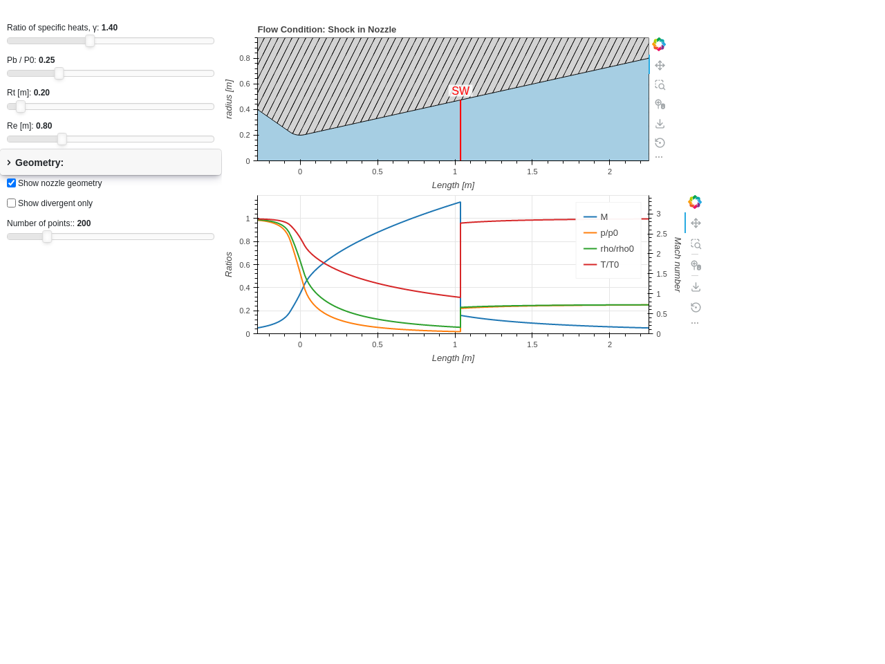
Visualize an interactive application:
from pygasflow.nozzles import CD_Conical_Nozzle
from pygasflow.solvers import De_Laval_Solver
Ri, Rt, Re = 0.4, 0.2, 0.8  # Inlet Radius, Throat Radius, Exit Radius
nozzle = CD_Conical_Nozzle(Ri, Re, Rt)
solver = De_Laval_Solver(
    gamma=1.4, R=287.05, T0=298, P0=101325,
    nozzle=nozzle, Pb_P0_ratio=0.25)
solver.plot()
- property critical_area
Returns the critical area
- property inlet_area
Returns the inlet area
- property outlet_area
Returns the outlet area
- plot(interactive=True, show_nozzle=True, **params)[source]
Visualize the results.
- Parameters:
- interactivebool
If True, returns an interactive application in the form of a servable object, which will be automatically rendered inside a Jupyter Notebook. If any other interpreter is used, then
solver.plot(interactive=True).show()might be requires in order to visualize the application on a browser. If False, a Bokeh figure will be shown on the screen.- show_nozzlebool
- **params
Keyword arguments sent to
DeLavalDiagram.
- Returns:
- app
The application or figure to be shown.
Gas Related Solvers
- pygasflow.solvers.gas.gas_solver(p1_name, p1_value, p2_name='gamma', p2_value=1.4, to_dict=None)[source]
For a thermally perfect gas, compute quantities like the ratio of specific heats, the heat capacities and the mass-specific gas constant.
- Parameters:
- p1_namestr
Name of the first parameter given in input. Can be either one of:
"cp": heat capacity at constant pressure."cv": heat capacity at constant volume."gamma": ration of specific heats."r": mass-specific gas constant.
- p1_valuefloat
Actual value of the first parameter.
- p2_namestr
Name of the second parameter given in input. Can be either one of:
"cp": heat capacity at constant pressure."cv": heat capacity at constant volume."gamma": ration of specific heats."r": mass-specific gas constant.
It must be different from
p1_name.- p2_valuefloat
Actual value of the second parameter.
- to_dictbool, optional
If False, the function returns a list of results. If True, it returns a dictionary in which the keys are listed in the Returns section. Default to False (return a list of results).
- Returns:
- gammafloat
- rfloat
- Cpfloat
- Cvfloat
See also
Examples
Compute the specific heats for air:
>>> from pygasflow.solvers.gas import gas_solver
>>> res1 = gas_solver("r", 287.05, "gamma", 1.4)
>>> res1
[1.4, 287.05, 1004.6750000000002, 717.6250000000002]
>>> res1.show()
idx   quantity
-------------------
0     gamma             1.40000000
1     R               287.05000000
2     Cp             1004.67500000
3     Cv              717.62500000
Compute the specific heats for methane, using pint quantities:
>>> import pint
>>> ureg = pint.UnitRegistry()
>>> res2 = gas_solver(
...     "r", 518.28 * ureg.J / (ureg.kg * ureg.K), "gamma", 1.32,
...     to_dict=True)
>>> res2
{'gamma': 1.32, 'R': <Quantity(518.28, 'joule / kilogram / kelvin')>, 'Cp': <Quantity(2137.905, 'joule / kilogram / kelvin')>, 'Cv': <Quantity(1619.625, 'joule / kilogram / kelvin')>}
>>> res2.show()
key     quantity
-------------------------
gamma   gamma                 1.32000000
R       R [J / K / kg]      518.28000000
Cp      Cp [J / K / kg]    2137.90500000
Cv      Cv [J / K / kg]    1619.62500000
- pygasflow.solvers.gas.print_gas_results(results, number_formatter=None, blank_line=False)[source]
- Parameters:
- resultslist or dict
- number_formatterstr or None
A formatter to properly show floating point numbers. For example,
"{:>8.3f}"to show numbers with 3 decimal places.- blank_linebool
If True, a blank line will be printed after the results.
See also
- pygasflow.solvers.gas.ideal_gas_solver(wanted, p=None, rho=None, R=None, T=None, to_dict=None)[source]
Solve for quantities of the ideal gas law: p/rho = R*T
Note: 3 numerical parameters are needed to compute the wanted quantity.
- Parameters:
- wantedstr
Name of the parameter to compute. Can be either one of:
"p": static pressure [Pa]."rho": density [Kg / m**3]."R": mass-specific gas constant [J / (Kg K)]."T": temperature [K].
- pfloat or None
Static pressure [Pa].
- rhofloat or None
Density [Kg / m**3].
- Rfloat or None
Mass-specific gas constant [J / (Kg K)].
- Tfloat or None
Temperature [K].
- to_dictbool, optional
If False, the function returns a list of results. If True, it returns a dictionary in which the keys are listed in the Returns section. Default to False.
- Returns:
- pfloat
- rhofloat
- Rfloat
- Tfloat
See also
print_ideal_gas_resultsIdealGasDiagram
Examples
>>> from pygasflow.solvers.gas import ideal_gas_solver
>>> res1 = ideal_gas_solver("p", R=287.05, T=288, rho=1.2259)
>>> res1
[101345.64336000002, 1.2259, 287.05, 288]
>>> res1.show()
idx   quantity
-------------------
0     P            101345.64336000
1     rho               1.22590000
2     R               287.05000000
3     T               288.00000000
>>> res2 = ideal_gas_solver("p", R=287.05, T=288, rho=1.2259, to_dict=True)
>>> res2
{'p': 101345.64336000002, 'rho': 1.2259, 'R': 287.05, 'T': 288}
>>> res2.show()
key     quantity
---------------------
p       P            101345.64336000
rho     rho               1.22590000
R       R               287.05000000
T       T               288.00000000
- pygasflow.solvers.gas.print_ideal_gas_results(results, number_formatter=None, blank_line=False)[source]
- Parameters:
- resultslist or dict
- number_formatterstr or None
A formatter to properly show floating point numbers. For example,
"{:>8.3f}"to show numbers with 3 decimal places.- blank_linebool
If True, a blank line will be printed after the results.
See also
- pygasflow.solvers.gas.sonic_condition(gamma=1.4, to_dict=False)[source]
Compute the sonic condition for a gas.
- Parameters:
- gammafloat, optional
Specific heats ratio. Default to 1.4. Must be \(\gamma > 1\).
- to_dictbool, optional
If False, the function returns a list of results. If True, it returns a dictionary in which the keys are listed in the Returns section. Default to False (return a list of results).
- Returns:
- drsfloat
Sonic density ratio rho0/rho*
- prsfloat
Sonic pressure ratio P0/P*
- arsfloat
Sonic Temperature ratio a0/a*
- trsfloat
Sonic Temperature ratio T0/T*
Examples
>>> from pygasflow.solvers import sonic_condition
>>> res = sonic_condition(1.4, to_dict=True)
>>> res
{'drs': np.float64(1.5774409656148785), 'prs': np.float64(1.892929158737854), 'ars': np.float64(1.0954451150103321), 'trs': np.float64(1.2)}
>>> res.show()
key     quantity
---------------------
drs     rho0/rho*         1.57744097
prs     P0/P*             1.89292916
ars     a0/T*             1.09544512
trs     T0/T*             1.20000000
- pygasflow.solvers.gas.print_sonic_condition_results(results, number_formatter=None, blank_line=False)[source]
- Parameters:
- resultslist or dict
- number_formatterstr or None
A formatter to properly show floating point numbers. For example,
"{:>8.3f}"to show numbers with 3 decimal places.- blank_linebool
If True, a blank line will be printed after the results.
See also