Interactive

Objectives of the interactive modules:

1. to have a web-based GUI (Graphical User Interface) always available to the user.

2. to simplify even further the use of pygasflow.

3. to make parametric visualizations easier than ever, thus improving the learning experience about quasi-1D ideal gasdynamic.

The interactive module is built with Holoviz Param and Panel. It is composed of several components:

• Diagrams, used to visualize the general results of a particular solver.

• Tabulators, used to visualize dataframes containing the numerical results of a particular solver.

• Sections, composed of diagrams and/or tabulators.

• Pages (or tabs), composed of different sections.

• Overall application, composed of different pages (or tabs).

The following are the most important functions available to the users.

Applications

pygasflow.interactive.compressible_app(theme='default')

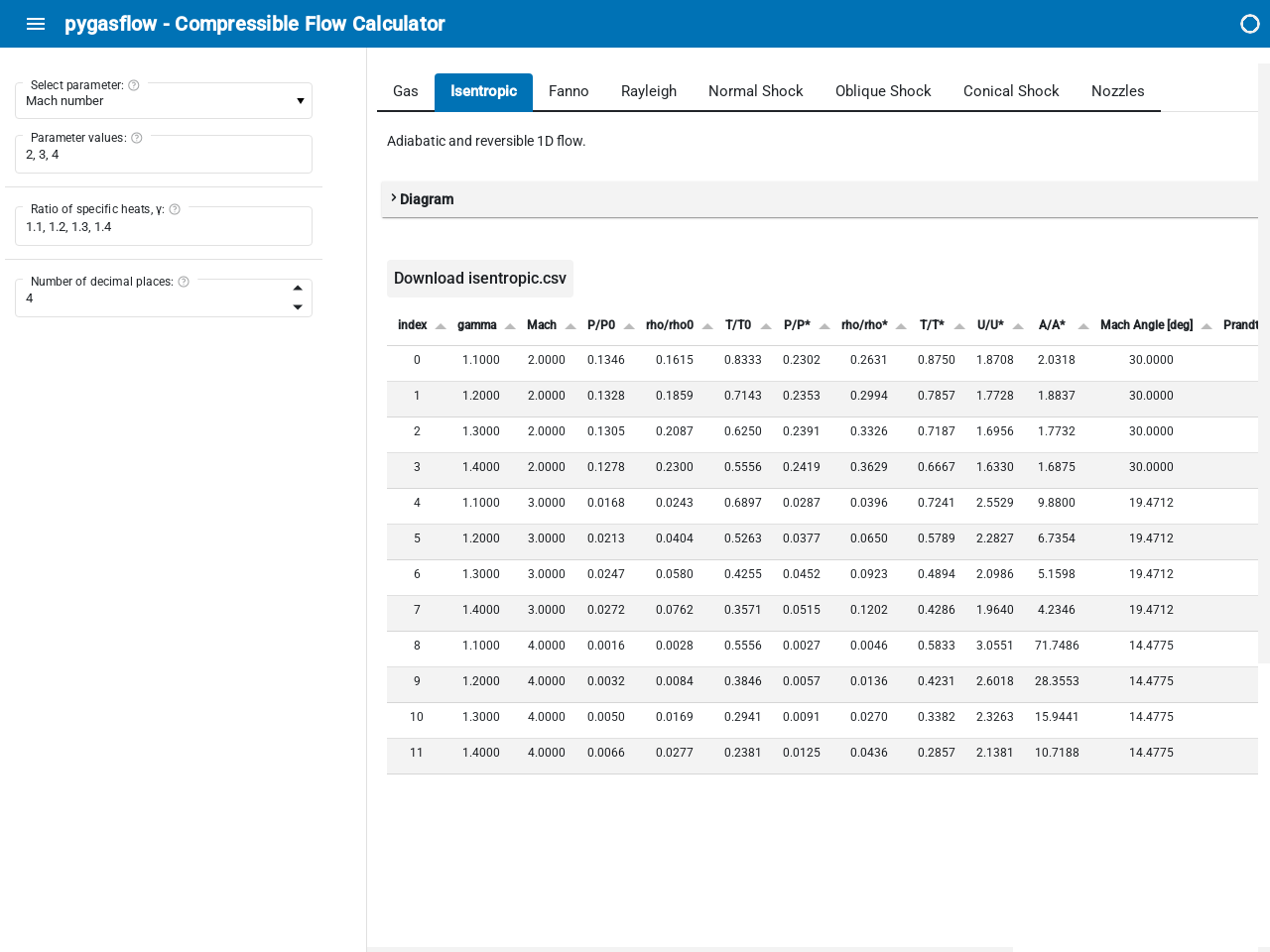
Create the ‘Compressible Flow Calculator’ web application.

Note that while the application works on a browser, all the computation is done with Python and the pygasflow module.

Parameters:

themestr

Can be "default" (light theme) or "dark" for using a dark theme.

Examples

Launching a server from a command line. This is the content of a user-created file, pygasflow_gui.py:

from pygasflow.interactive import compressible_app
compressible_app().servable()

Then, from the command line:

panel serve pygasflow_gui.py

Launching a server from Jupyter Notebook:

from pygasflow.interactive import compressible_app
app = compressible_app()
app.show()

(Source code, large.png)

Diagrams

class pygasflow.interactive.diagrams.IsentropicDiagram(*, angle_lines_kwargs, ratio_lines_kwargs, select, y_label_right, y_range_right, _parameter_name, _solver, mach_range, tooltips, N, gamma, labels, results, _theme, _update_func, colors, error_log, figure, legend, show_legend_outside, show_minor_grid, size, title, x_label, x_range, y_label, y_range, name)

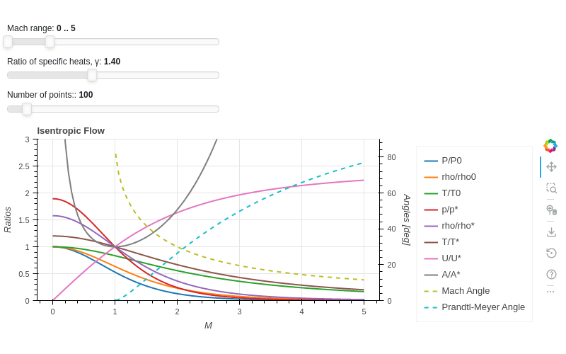
Interactive component to create a diagram for the isentropic flow.

Parameters:

figurebokeh.plotting._figure.figure

allow_None:

True

The Bokeh figure to populate

sizeTuple

allow_None:

True

default:

(800, 300)

length:

2

Size of the plot, (width, height) in pixel.

error_logString

default:

Visualize any error that raises from the computation.

colorsTuple

default:

(‘#1f77b4’, ‘#ff7f0e’, ‘#2ca02c’, ‘#d62728’, ‘#9467bd’, ‘#8c564b’, ‘#e377c2’, ‘#7f7f7f’, ‘#bcbd22’, ‘#17becf’)

length:

10

List of categorical colors.

legendbokeh.models.annotations.legends.Legend

allow_None:

True

The legend, when placed outside of the plotting area.

titleString

default:

x_labelString

default:

M

y_labelString

default:

Ratios

x_rangeRange

allow_None:

True

inclusive_bounds:

(True, True)

length:

2

y_rangeRange

allow_None:

True

inclusive_bounds:

(True, True)

length:

2

show_minor_gridBoolean

default:

False

Toggle minor grid visibility.

show_legend_outsideBoolean

default:

True

If True, the legend will be moved outside of the plotting area. In doing so, the legend items will become clickable, allowing user to hide a particular line.

gammaNumber

bounds:

gamma >= 1

default:

1.4

γ = Cp / Cv

NInteger

bounds:

N >= 10

default:

100

Number of points for each curve. It affects the quality of the visualization as well as the speed of updates.

labelsList

default:

[]

Labels to be used on the legend.

resultsList

default:

[]

Results of the computation.

mach_rangeRange

bounds:

(0, 25)

default:

(0, 5)

inclusive_bounds:

(True, True)

length:

2

Minimum and Maximum Mach number for the visualization.

tooltipsList

default:

[(‘Variable’, ‘@v’), (‘Mach’, ‘@xs’), (‘value’, ‘@ys’)]

Tooltips used on each line of the plot.

y_label_rightString

default:

Angles [deg]

y_range_rightRange

bounds:

(0, 25)

default:

(0, 3)

inclusive_bounds:

(True, True)

length:

2

selectSelector

default:

1

names:

{‘Ratios + Angles’: 0, ‘Ratios’: 1, ‘Angles’: 2}

objects:

[0, 1, 2]

Chose which diagram to show.

angle_lines_kwargsDict

default:

{}

Keyword arguments to customize the appearance of the Mach Angle and Prandtl-Meyer Angle.

ratio_lines_kwargsDict

default:

{}

Keyword arguments to customize the appearance of the ratios.

Examples

Show an interactive application:

from pygasflow.interactive.diagrams import IsentropicDiagram
IsentropicDiagram()

(Source code, large.png)

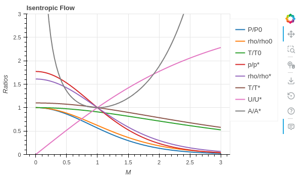
Set custom values to parameters and only show the figure about the ratios:

from pygasflow.interactive.diagrams import IsentropicDiagram
d = IsentropicDiagram(
    select=1,
    mach_range=(0, 3),
    gamma=1.2,
    size=(600, 350)
)
d.show_figure()

(Source code, large.png)

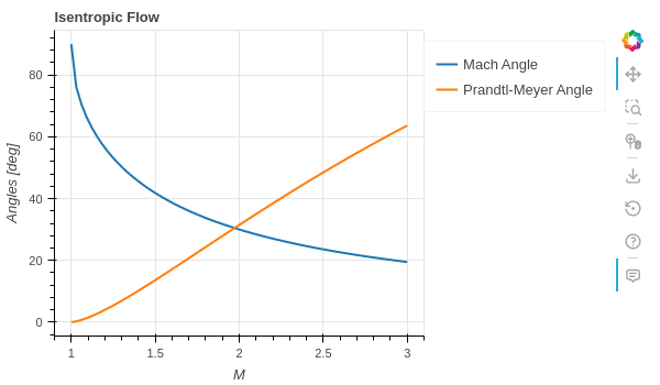
Set custom values to parameters and only show the figure about the angles:

from pygasflow.interactive.diagrams import IsentropicDiagram
d = IsentropicDiagram(
    select=2,
    mach_range=(0, 3),
    gamma=1.2,
    size=(600, 350),
    angle_lines_kwargs={"line_dash": "solid"}
)
d.show_figure()

(Source code, large.png)

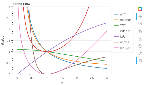
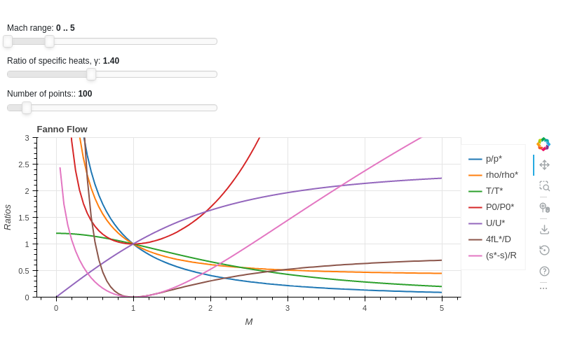
class pygasflow.interactive.diagrams.FannoDiagram(*, _parameter_name, _solver, mach_range, tooltips, N, gamma, labels, results, _theme, _update_func, colors, error_log, figure, legend, show_legend_outside, show_minor_grid, size, title, x_label, x_range, y_label, y_range, name)

Interactive component to create a diagram for the Fanno flow, ie the 1D flow with head addition.

Parameters:

figurebokeh.plotting._figure.figure

allow_None:

True

The Bokeh figure to populate

sizeTuple

allow_None:

True

default:

(800, 300)

length:

2

Size of the plot, (width, height) in pixel.

error_logString

default:

Visualize any error that raises from the computation.

colorsTuple

default:

(‘#1f77b4’, ‘#ff7f0e’, ‘#2ca02c’, ‘#d62728’, ‘#9467bd’, ‘#8c564b’, ‘#e377c2’, ‘#7f7f7f’, ‘#bcbd22’, ‘#17becf’)

length:

10

List of categorical colors.

legendbokeh.models.annotations.legends.Legend

allow_None:

True

The legend, when placed outside of the plotting area.

titleString

default:

x_labelString

default:

M

y_labelString

default:

Ratios

x_rangeRange

allow_None:

True

inclusive_bounds:

(True, True)

length:

2

y_rangeRange

allow_None:

True

inclusive_bounds:

(True, True)

length:

2

show_minor_gridBoolean

default:

False

Toggle minor grid visibility.

show_legend_outsideBoolean

default:

True

If True, the legend will be moved outside of the plotting area. In doing so, the legend items will become clickable, allowing user to hide a particular line.

gammaNumber

bounds:

gamma >= 1

default:

1.4

γ = Cp / Cv

NInteger

bounds:

N >= 10

default:

100

Number of points for each curve. It affects the quality of the visualization as well as the speed of updates.

labelsList

default:

[]

Labels to be used on the legend.

resultsList

default:

[]

Results of the computation.

mach_rangeRange

bounds:

(0, 25)

default:

(0, 5)

inclusive_bounds:

(True, True)

length:

2

Minimum and Maximum Mach number for the visualization.

tooltipsList

default:

[(‘Variable’, ‘@v’), (‘Mach’, ‘@xs’), (‘value’, ‘@ys’)]

Tooltips used on each line of the plot.

Examples

Show an interactive application:

from pygasflow.interactive.diagrams import FannoDiagram
FannoDiagram()

(Source code, large.png)

Set custom values to parameters and only show the figure:

from pygasflow.interactive.diagrams import FannoDiagram
d = FannoDiagram(mach_range=(0, 3), gamma=1.2, size=(600, 350))
d.show_figure()

(Source code, large.png)

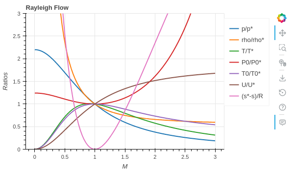
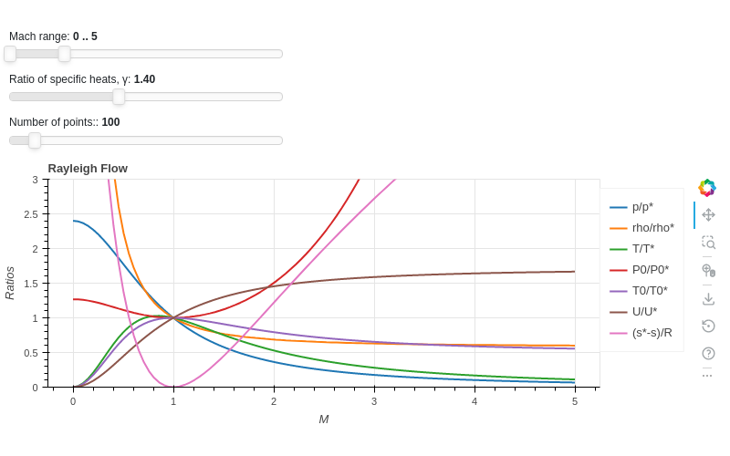
class pygasflow.interactive.diagrams.RayleighDiagram(*, _parameter_name, _solver, mach_range, tooltips, N, gamma, labels, results, _theme, _update_func, colors, error_log, figure, legend, show_legend_outside, show_minor_grid, size, title, x_label, x_range, y_label, y_range, name)

Interactive component to create a diagram for the Rayleigh flow, ie the 1D flow with friction.

Parameters:

figurebokeh.plotting._figure.figure

allow_None:

True

The Bokeh figure to populate

sizeTuple

allow_None:

True

default:

(800, 300)

length:

2

Size of the plot, (width, height) in pixel.

error_logString

default:

Visualize any error that raises from the computation.

colorsTuple

default:

(‘#1f77b4’, ‘#ff7f0e’, ‘#2ca02c’, ‘#d62728’, ‘#9467bd’, ‘#8c564b’, ‘#e377c2’, ‘#7f7f7f’, ‘#bcbd22’, ‘#17becf’)

length:

10

List of categorical colors.

legendbokeh.models.annotations.legends.Legend

allow_None:

True

The legend, when placed outside of the plotting area.

titleString

default:

x_labelString

default:

M

y_labelString

default:

Ratios

x_rangeRange

allow_None:

True

inclusive_bounds:

(True, True)

length:

2

y_rangeRange

allow_None:

True

inclusive_bounds:

(True, True)

length:

2

show_minor_gridBoolean

default:

False

Toggle minor grid visibility.

show_legend_outsideBoolean

default:

True

If True, the legend will be moved outside of the plotting area. In doing so, the legend items will become clickable, allowing user to hide a particular line.

gammaNumber

bounds:

gamma >= 1

default:

1.4

γ = Cp / Cv

NInteger

bounds:

N >= 10

default:

100

Number of points for each curve. It affects the quality of the visualization as well as the speed of updates.

labelsList

default:

[]

Labels to be used on the legend.

resultsList

default:

[]

Results of the computation.

mach_rangeRange

bounds:

(0, 25)

default:

(0, 5)

inclusive_bounds:

(True, True)

length:

2

Minimum and Maximum Mach number for the visualization.

tooltipsList

default:

[(‘Variable’, ‘@v’), (‘Mach’, ‘@xs’), (‘value’, ‘@ys’)]

Tooltips used on each line of the plot.

Examples

Show an interactive application:

from pygasflow.interactive.diagrams import RayleighDiagram
RayleighDiagram()

(Source code, large.png)

Set custom values to parameters and only show the figure:

from pygasflow.interactive.diagrams import RayleighDiagram
d = RayleighDiagram(mach_range=(0, 3), gamma=1.2, size=(600, 350))
d.show_figure()

(Source code, large.png)

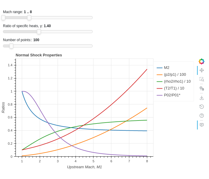
class pygasflow.interactive.diagrams.NormalShockDiagram(*, dividers, _parameter_name, _solver, mach_range, tooltips, N, gamma, labels, results, _theme, _update_func, colors, error_log, figure, legend, show_legend_outside, show_minor_grid, size, title, x_label, x_range, y_label, y_range, name)

Interactive component to create a diagram for the properties of the flow as it crosses a normal shock wave.

Parameters:

figurebokeh.plotting._figure.figure

allow_None:

True

The Bokeh figure to populate

sizeTuple

allow_None:

True

default:

(800, 300)

length:

2

Size of the plot, (width, height) in pixel.

error_logString

default:

Visualize any error that raises from the computation.

colorsTuple

default:

(‘#1f77b4’, ‘#ff7f0e’, ‘#2ca02c’, ‘#d62728’, ‘#9467bd’, ‘#8c564b’, ‘#e377c2’, ‘#7f7f7f’, ‘#bcbd22’, ‘#17becf’)

length:

10

List of categorical colors.

legendbokeh.models.annotations.legends.Legend

allow_None:

True

The legend, when placed outside of the plotting area.

titleString

default:

x_labelString

default:

M

y_labelString

default:

Ratios

x_rangeRange

allow_None:

True

inclusive_bounds:

(True, True)

length:

2

y_rangeRange

allow_None:

True

inclusive_bounds:

(True, True)

length:

2

show_minor_gridBoolean

default:

False

Toggle minor grid visibility.

show_legend_outsideBoolean

default:

True

If True, the legend will be moved outside of the plotting area. In doing so, the legend items will become clickable, allowing user to hide a particular line.

gammaNumber

bounds:

gamma >= 1

default:

1.4

γ = Cp / Cv

NInteger

bounds:

N >= 10

default:

100

Number of points for each curve. It affects the quality of the visualization as well as the speed of updates.

labelsList

default:

[]

Labels to be used on the legend.

resultsList

default:

[]

Results of the computation.

mach_rangeRange

bounds:

(1, 25)

default:

(1, 8)

inclusive_bounds:

(True, True)

length:

2

Minimum and Maximum Mach number for the visualization.

tooltipsList

default:

[(‘Variable’, ‘@v’), (‘Mach’, ‘@xs’), (‘value’, ‘@ys’)]

Tooltips used on each line of the plot.

dividersList

default:

[1, 100, 10, 10, 1]

Some ratios are going to be much bigger than others at the same upstream Mach number. Each number of this list represents a quotient for a particular ratio in order to “normalize” the visualization.

Examples

Show an interactive application:

from pygasflow.interactive.diagrams import NormalShockDiagram
NormalShockDiagram()

(Source code, large.png)

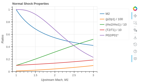
Set custom values to parameters and only show the figure:

from pygasflow.interactive.diagrams import NormalShockDiagram
d = NormalShockDiagram(
    mach_range=(1, 3), gamma=1.2, size=(600, 350), y_range=(0, 1.05))
d.show_figure()

(Source code, large.png)

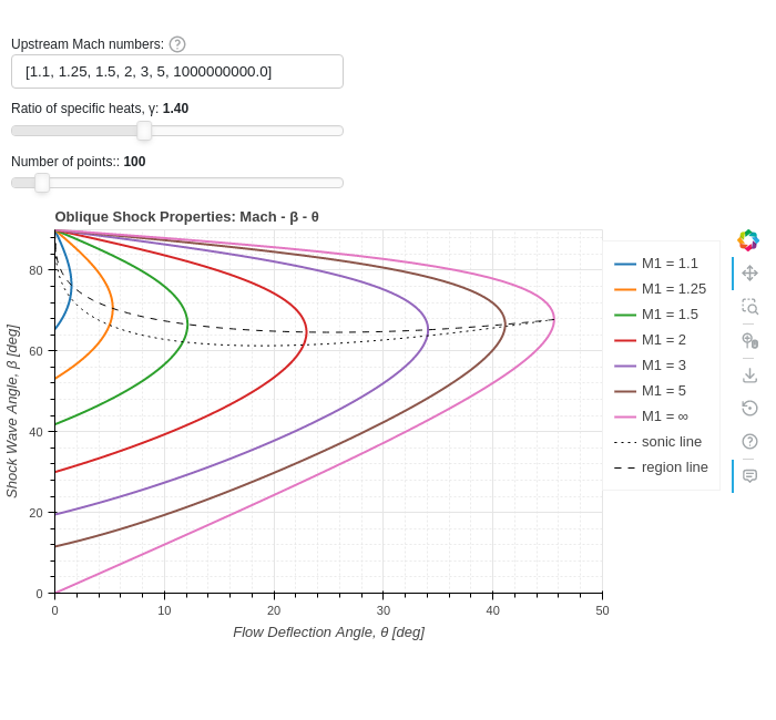
class pygasflow.interactive.diagrams.ObliqueShockDiagram(*, _additional_mach_lines, _region_line, _sonic_line, _upstream_mach_lines, add_region_line, add_sonic_line, add_upstream_mach, additional_upstream_mach, tooltips, upstream_mach, N, gamma, labels, results, _theme, _update_func, colors, error_log, figure, legend, show_legend_outside, show_minor_grid, size, title, x_label, x_range, y_label, y_range, name)

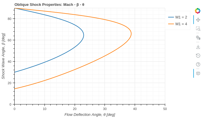
Interactive component to create a diagram for the properties of the flow as it crosses an oblique shock wave.

Parameters:

figurebokeh.plotting._figure.figure

allow_None:

True

The Bokeh figure to populate

sizeTuple

allow_None:

True

default:

(800, 300)

length:

2

Size of the plot, (width, height) in pixel.

error_logString

default:

Visualize any error that raises from the computation.

colorsTuple

default:

(‘#1f77b4’, ‘#ff7f0e’, ‘#2ca02c’, ‘#d62728’, ‘#9467bd’, ‘#8c564b’, ‘#e377c2’, ‘#7f7f7f’, ‘#bcbd22’, ‘#17becf’)

length:

10

List of categorical colors.

legendbokeh.models.annotations.legends.Legend

allow_None:

True

The legend, when placed outside of the plotting area.

titleString

default:

x_labelString

default:

M

y_labelString

default:

Ratios

x_rangeRange

allow_None:

True

inclusive_bounds:

(True, True)

length:

2

y_rangeRange

allow_None:

True

inclusive_bounds:

(True, True)

length:

2

show_minor_gridBoolean

default:

False

Toggle minor grid visibility.

show_legend_outsideBoolean

default:

True

If True, the legend will be moved outside of the plotting area. In doing so, the legend items will become clickable, allowing user to hide a particular line.

gammaNumber

bounds:

gamma >= 1

default:

1.4

γ = Cp / Cv

NInteger

bounds:

N >= 10

default:

100

Number of points for each curve. It affects the quality of the visualization as well as the speed of updates.

labelsList

default:

[]

Labels to be used on the legend.

resultsList

default:

[]

Results of the computation.

upstream_machList

length:

7

default:

[1.1, 1.5, 2, 3, 5, 10, 1000000000.0]

item_type:

(float, int)

Comma separated list of 7 upstream Mach numbers to be shown.

additional_upstream_machList

default:

[]

item_type:

numbers.Number

User can provides additional upstream Mach numbers to be plotted on the chart. This parameter must be set at instantiation and should be changed afterwards.

add_upstream_machBoolean

default:

True

If True, add the default upstream Mach numbers to the chart. Otherwise, only add the additional user-provided Mach numbers. This parameter must be set at instantiation and should be changed afterwards.

add_sonic_lineBoolean

default:

True

Add the line where the downstream Mach number is M2=1. This parameter must be set at instantiation and should be changed afterwards.

add_region_lineBoolean

default:

True

Add the line separating the strong solution from the weak solution. This parameter must be set at instantiation and should be changed afterwards.

tooltipsList

default:

[(‘Variable’, ‘@v’), (‘θ’, ‘@x’), (‘β’, ‘@y’), (‘Region’, ‘@r’)]

Tooltips used on each line of the plot.

Examples

Show an interactive application:

from pygasflow.interactive.diagrams import ObliqueShockDiagram
ObliqueShockDiagram()

(Source code, large.png)

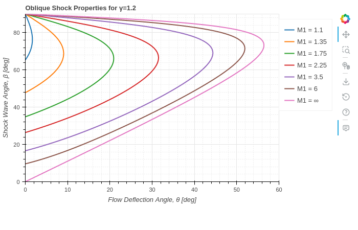
Set custom values to parameters, hide sonic and region lines, and only show the figure:

from pygasflow.interactive.diagrams import ObliqueShockDiagram
d = ObliqueShockDiagram(
    upstream_mach=[1.1, 1.35, 1.75, 2.25, 3.5, 6, 1e06],
    gamma=1.2,
    add_region_line=False,
    add_sonic_line=False,
    title="Oblique Shock Properties for γ=1.2",
    N=1000
)
d.show_figure()

(Source code, large.png)

Only shows user-specified upstream Mach numbers:

from pygasflow.interactive.diagrams import ObliqueShockDiagram
d = ObliqueShockDiagram(
    add_upstream_mach=False,
    add_region_line=False,
    add_sonic_line=False,
    additional_upstream_mach=[2, 4],
)
d.show_figure()

(Source code, large.png)

class pygasflow.interactive.diagrams.ConicalShockDiagram(*, _additional_mach_lines, _region_line, _sonic_line, _upstream_mach_lines, add_region_line, add_sonic_line, add_upstream_mach, additional_upstream_mach, tooltips, upstream_mach, N, gamma, labels, results, _theme, _update_func, colors, error_log, figure, legend, show_legend_outside, show_minor_grid, size, title, x_label, x_range, y_label, y_range, name)

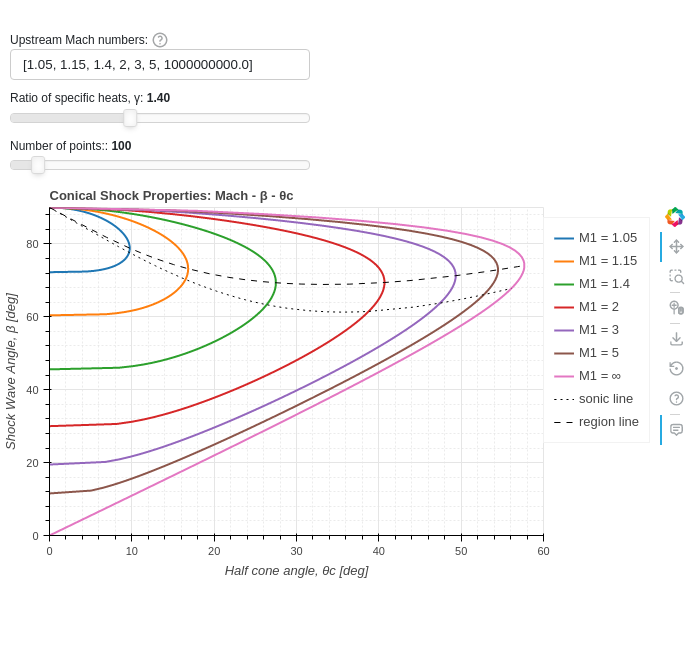
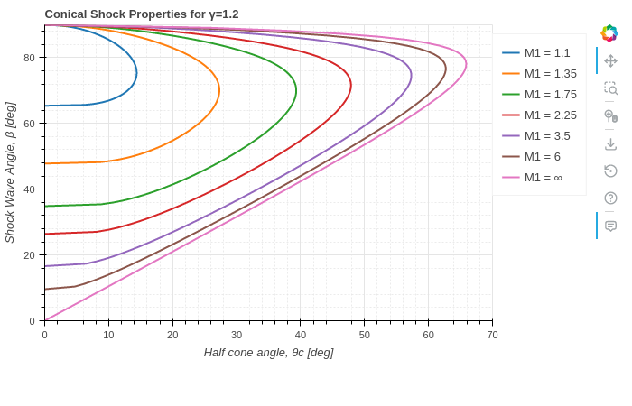
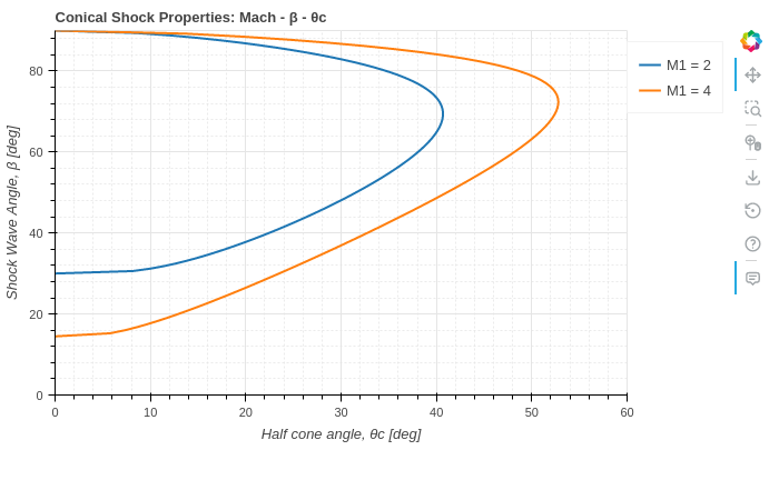
Interactive component to create a diagram for the properties of the axisymmetric supersonic flow over a sharp cone at zero angle of attack to the free stream.

Parameters:

figurebokeh.plotting._figure.figure

allow_None:

True

The Bokeh figure to populate

sizeTuple

allow_None:

True

default:

(800, 300)

length:

2

Size of the plot, (width, height) in pixel.

error_logString

default:

Visualize any error that raises from the computation.

colorsTuple

default:

(‘#1f77b4’, ‘#ff7f0e’, ‘#2ca02c’, ‘#d62728’, ‘#9467bd’, ‘#8c564b’, ‘#e377c2’, ‘#7f7f7f’, ‘#bcbd22’, ‘#17becf’)

length:

10

List of categorical colors.

legendbokeh.models.annotations.legends.Legend

allow_None:

True

The legend, when placed outside of the plotting area.

titleString

default:

x_labelString

default:

M

y_labelString

default:

Ratios

x_rangeRange

allow_None:

True

inclusive_bounds:

(True, True)

length:

2

y_rangeRange

allow_None:

True

inclusive_bounds:

(True, True)

length:

2

show_minor_gridBoolean

default:

False

Toggle minor grid visibility.

show_legend_outsideBoolean

default:

True

If True, the legend will be moved outside of the plotting area. In doing so, the legend items will become clickable, allowing user to hide a particular line.

gammaNumber

bounds:

gamma >= 1

default:

1.4

γ = Cp / Cv

NInteger

bounds:

N >= 10

default:

100

Number of points for each curve. It affects the quality of the visualization as well as the speed of updates.

labelsList

default:

[]

Labels to be used on the legend.

resultsList

default:

[]

Results of the computation.

upstream_machList

length:

7

default:

[1.1, 1.5, 2, 3, 5, 10, 1000000000.0]

item_type:

(float, int)

Comma separated list of 7 upstream Mach numbers to be shown.

additional_upstream_machList

default:

[]

item_type:

numbers.Number

User can provides additional upstream Mach numbers to be plotted on the chart. This parameter must be set at instantiation and should be changed afterwards.

add_upstream_machBoolean

default:

True

If True, add the default upstream Mach numbers to the chart. Otherwise, only add the additional user-provided Mach numbers. This parameter must be set at instantiation and should be changed afterwards.

add_sonic_lineBoolean

default:

True

Add the line where the downstream Mach number is M2=1. This parameter must be set at instantiation and should be changed afterwards.

add_region_lineBoolean

default:

True

Add the line separating the strong solution from the weak solution. This parameter must be set at instantiation and should be changed afterwards.

tooltipsList

default:

[(‘Variable’, ‘@v’), (‘θ’, ‘@x’), (‘β’, ‘@y’), (‘Region’, ‘@r’)]

Tooltips used on each line of the plot.

Examples

Show an interactive application:

from pygasflow.interactive.diagrams import ConicalShockDiagram
ConicalShockDiagram()

(Source code, large.png)

Set custom values to parameters, hide sonic and region lines, and only show the figure:

from pygasflow.interactive.diagrams import ConicalShockDiagram
d = ConicalShockDiagram(
    upstream_mach=[1.1, 1.35, 1.75, 2.25, 3.5, 6, 1e06],
    gamma=1.2,
    add_region_line=False,
    add_sonic_line=False,
    title="Conical Shock Properties for γ=1.2"
)
d.show_figure()

(Source code, large.png)

Only shows user-specified upstream Mach numbers:

from pygasflow.interactive.diagrams import ConicalShockDiagram
d = ConicalShockDiagram(
    add_upstream_mach=False,
    add_region_line=False,
    add_sonic_line=False,
    additional_upstream_mach=[2, 4],
)
d.show_figure()

(Source code, large.png)

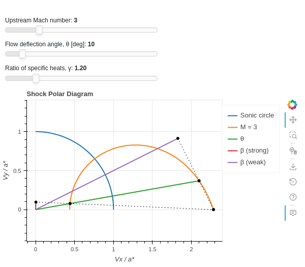
class pygasflow.interactive.diagrams.ShockPolarDiagram(*, _beta_strong_line, _beta_weak_line, _helper_line_1, _helper_line_2, _helper_line_3, _helper_line_4, _helper_scatter_1, _helper_scatter_22, _helper_scatter_3, _helper_scatter_4, _mach_inf, _mach_line, _sonic_circle, _theta_line, characteristic_mach_number, helper_line_kwargs, helper_scatter_kwargs, include_mirror, mach_number, show_beta_line, show_mach_at_infinity, show_sonic_circle, show_theta_line, theta, theta_max, N, gamma, labels, results, _theme, _update_func, colors, error_log, figure, legend, show_legend_outside, show_minor_grid, size, title, x_label, x_range, y_label, y_range, name)

Create a shock polar diagram.

Parameters:

figurebokeh.plotting._figure.figure

allow_None:

True

The Bokeh figure to populate

sizeTuple

allow_None:

True

default:

(800, 300)

length:

2

Size of the plot, (width, height) in pixel.

error_logString

default:

Visualize any error that raises from the computation.

colorsTuple

default:

(‘#1f77b4’, ‘#ff7f0e’, ‘#2ca02c’, ‘#d62728’, ‘#9467bd’, ‘#8c564b’, ‘#e377c2’, ‘#7f7f7f’, ‘#bcbd22’, ‘#17becf’)

length:

10

List of categorical colors.

legendbokeh.models.annotations.legends.Legend

allow_None:

True

The legend, when placed outside of the plotting area.

titleString

default:

x_labelString

default:

M

y_labelString

default:

Ratios

x_rangeRange

allow_None:

True

inclusive_bounds:

(True, True)

length:

2

y_rangeRange

allow_None:

True

inclusive_bounds:

(True, True)

length:

2

show_minor_gridBoolean

default:

False

Toggle minor grid visibility.

show_legend_outsideBoolean

default:

True

If True, the legend will be moved outside of the plotting area. In doing so, the legend items will become clickable, allowing user to hide a particular line.

gammaNumber

bounds:

gamma >= 1

default:

1.4

γ = Cp / Cv

NInteger

bounds:

N >= 10

default:

100

Number of points for each curve. It affects the quality of the visualization as well as the speed of updates.

labelsList

default:

[]

Labels to be used on the legend.

resultsList

default:

[]

Results of the computation.

show_mach_at_infinityBoolean

default:

False

Toggle the visibility of the curve at Mach infinity.

show_theta_lineBoolean

default:

True

Show the line representing the deflection angle, θ.

show_beta_lineBoolean

default:

True

Show the line representing the shock wave angle, β.

show_sonic_circleBoolean

default:

True

Show the line representing the sonic circle.

mach_numberNumber

bounds:

mach_number >= 1

default:

5

Mach number to represent on the diagram.

thetaNumber

bounds:

\(0 \le \theta \le 90\)

default:

15

Flow deflection angle, θ [deg]

include_mirrorBoolean

default:

False

If True, shows results both on +Y and -Y axis.

characteristic_mach_numberNumber

read only:

True

Get the characteristic upstream Mach number.

theta_maxNumber

read only:

True

Get the maximum deflection angle associated with the current upstream Mach number.

helper_line_kwargsDict

default:

{}

Rendering keywords for helper lines.

helper_scatter_kwargsDict

default:

{}

Rendering keywords for helper lines.

Examples

Show an interactive application:

from pygasflow.interactive.diagrams import ShockPolarDiagram
ShockPolarDiagram(mach_number=3, gamma=1.2, theta=10)

(Source code, large.png)

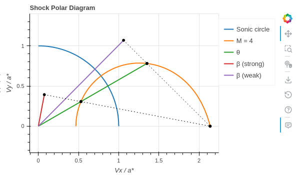
Set custom values to parameters and only show the figure:

from pygasflow.interactive.diagrams import ShockPolarDiagram
d = ShockPolarDiagram(mach_number=4, gamma=1.4, theta=30)
d.show_figure()

(Source code, large.png)

class pygasflow.interactive.diagrams.PressureDeflectionDiagram(*, _theme, _update_func, colors, error_log, figure, legend, show_legend_outside, show_minor_grid, size, title, x_label, x_range, y_label, y_range, name)

Creates a pressure-deflection diagram.

Parameters:

figurebokeh.plotting._figure.figure

allow_None:

True

The Bokeh figure to populate

sizeTuple

allow_None:

True

default:

(800, 300)

length:

2

Size of the plot, (width, height) in pixel.

error_logString

default:

Visualize any error that raises from the computation.

colorsTuple

default:

(‘#1f77b4’, ‘#ff7f0e’, ‘#2ca02c’, ‘#d62728’, ‘#9467bd’, ‘#8c564b’, ‘#e377c2’, ‘#7f7f7f’, ‘#bcbd22’, ‘#17becf’)

length:

10

List of categorical colors.

legendbokeh.models.annotations.legends.Legend

allow_None:

True

The legend, when placed outside of the plotting area.

titleString

default:

x_labelString

default:

M

y_labelString

default:

Ratios

x_rangeRange

allow_None:

True

inclusive_bounds:

(True, True)

length:

2

y_rangeRange

allow_None:

True

inclusive_bounds:

(True, True)

length:

2

show_minor_gridBoolean

default:

False

Toggle minor grid visibility.

show_legend_outsideBoolean

default:

True

If True, the legend will be moved outside of the plotting area. In doing so, the legend items will become clickable, allowing user to hide a particular line.

Examples

from pygasflow.shockwave import PressureDeflectionLocus
from pygasflow.interactive import PressureDeflectionDiagram

M1 = 3
theta_2 = 20
theta_3 = -15

loc1 = PressureDeflectionLocus(M=M1, label="1")
loc2 = loc1.new_locus_from_shockwave(theta_2, label="2")
loc3 = loc1.new_locus_from_shockwave(theta_3, label="3")

phi, p4_p1 = loc2.intersection(loc3)
print("Intersection between locus M2 and locus M3 happens at:")
print("Deflection Angle [deg]:", phi)
print("Pressure ratio to freestream:", p4_p1)

d = PressureDeflectionDiagram(
    title="Intersection of shocks of opposite families"
)
d.add_locus(loc1)
d.add_locus(loc2)
d.add_locus(loc3)
d.add_path((loc1, theta_2), (loc2, phi))
d.add_path((loc1, theta_3), (loc3, phi))
d.add_state(
    phi, p4_p1, "4=4'",
    background_fill_color="white",
    background_fill_alpha=0.8)
d.move_legend_outside()
d.y_range = (0, 18)
d.show_figure()

(Source code, large.png)

add_locus(locus, show_state=True, N=100, include_mirror=True, **kwargs)

Add the locus to the diagram, with a single line.

Parameters:

locusPressureDeflectionLocus

show_statebool

If True, also add a text on the diagram at the start of the locus.

Nint

Number of discretization points.

include_mirrorbool

If False, only plot the locus for theta >= 0.

**kwargs

Keyword arguments passed to bokeh.models.Line

Returns:

line_rendbokeh.models.GlyphRenderer

lblbokeh.models.Label or None

circle_rendbokeh.models.GlyphRenderer or None

add_locus_split(locus, weak_kwargs={}, strong_kwargs={}, same_color=True, show_state=True, mode='region', N=100, include_mirror=True)

Add the locus to the diagram, with two lines, one for the weak region and the other for the strong region.

Parameters:

locusPressureDeflectionLocus

show_statebool

If True, also add a text on the diagram at the start of the locus.

weak_kwargsdict

Keyword arguments passed to bokeh.models.Line in order to customize the line for the weak region.

strong_kwargsdict

Keyword arguments passed to bokeh.models.Line in order to customize the line for the strong region.

same_colorbool

Wheter the two lines uses the same color.

show_statebool

If True, also add a text on the diagram at the start of the locus.

modestr

Split the locus at some point. It can be:

• "region": the locus is splitted at the detachment point, where theta=theta_max.

• "sonic": the locus is splitted at the sonic point (where the downstream Mach number is 1).

Nint

Number of discretization points.

include_mirrorbool

If False, only plot the locus for theta >= 0.

Returns:

line_rend_weakbokeh.models.GlyphRenderer

line_rend_strongbokeh.models.GlyphRenderer

lblbokeh.models.Label or None

circle_rendbokeh.models.GlyphRenderer or None

add_path(*segments, num_arrows=2, **kwargs)

Add a path connecting one or more segments.

Parameters:

segmentstuples

Each segment is a 2-elements tuple where the first element is a PressureDeflectionLocus, and the second element is the deflection angle [degrees] of the end of the segment.

num_arrowsint

Number of arrows to add over the each segment.

**kwargs

Keyword arguments passed to bokeh.models.Line.

Returns:

rendbokeh.models.GlyphRenderer

arrowsbokeh.models.Arrow

add_state(theta, pr, text, primary_line=None, circle_kw=None, **kwargs)

Add text to the specified point (x, y) in the diagram.

Parameters:

thetafloat

Flow deflection angle in degrees.

prfloat

Pressure ratio to freestream.

textstr

primary_lineNone or Renderer

If a Bokeh renderer is provided, its visibility will be linked to the label’s visibility. Useful to hide the label when the visibility of primary_line is toggled on the legend.

circle_kwNone or dict

Keyword arguments to bokeh.models.Circle.

**kwargs

Keyword arguments passed to bokeh.models.Label.

Returns:

lblbokeh.models.Label

circle_rendbokeh.models.GlyphRenderer

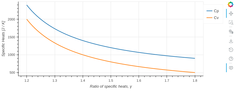
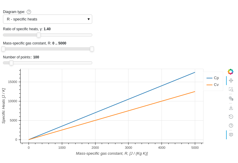
class pygasflow.interactive.diagrams.GasDiagram(*, N, R, R_range, gamma, gamma_range, select, _theme, _update_func, colors, error_log, figure, legend, show_legend_outside, show_minor_grid, size, title, x_label, x_range, y_label, y_range, name)

Plot the relationships Cp=f(gamma, R) and Cv=f(gamma, R).

Parameters:

figurebokeh.plotting._figure.figure

allow_None:

True

The Bokeh figure to populate

sizeTuple

allow_None:

True

default:

(800, 300)

length:

2

Size of the plot, (width, height) in pixel.

error_logString

default:

Visualize any error that raises from the computation.

colorsTuple

default:

(‘#1f77b4’, ‘#ff7f0e’, ‘#2ca02c’, ‘#d62728’, ‘#9467bd’, ‘#8c564b’, ‘#e377c2’, ‘#7f7f7f’, ‘#bcbd22’, ‘#17becf’)

length:

10

List of categorical colors.

legendbokeh.models.annotations.legends.Legend

allow_None:

True

The legend, when placed outside of the plotting area.

titleString

default:

x_labelString

default:

M

y_labelString

default:

Ratios

x_rangeRange

allow_None:

True

inclusive_bounds:

(True, True)

length:

2

y_rangeRange

allow_None:

True

inclusive_bounds:

(True, True)

length:

2

show_minor_gridBoolean

default:

False

Toggle minor grid visibility.

show_legend_outsideBoolean

default:

True

If True, the legend will be moved outside of the plotting area. In doing so, the legend items will become clickable, allowing user to hide a particular line.

selectSelector

default:

1

names:

{‘gamma - specific heats’: 0, ‘R - specific heats’: 1}

objects:

[0, 1]

Chose which diagram to show.

gammaNumber

bounds:

1 < gamma <= 2

default:

1.4

γ = Cp / Cv

gamma_rangeRange

bounds:

(1, 2)

default:

(1.05, 2)

inclusive_bounds:

(True, True)

length:

2

γ = Cp / Cv

RNumber

bounds:

0 <= R <= 5000

default:

287.05

[J / (Kg K)]

R_rangeRange

bounds:

(0, 5000)

default:

(0, 5000)

inclusive_bounds:

(True, True)

length:

2

[J / (Kg K)]

NInteger

bounds:

N >= 10

default:

100

Number of points for each curve. It affects the quality of the visualization as well as the speed of updates.

Examples

Show an interactive application:

from pygasflow.interactive.diagrams import GasDiagram
GasDiagram()

(Source code, large.png)

Set custom values to parameters and only show the figure:

from pygasflow.interactive.diagrams import GasDiagram
d = GasDiagram(select=0, gamma_range=(1.2, 1.8), R=400)
d.show_figure()

(Source code, large.png)

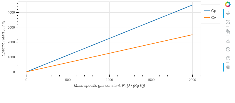
from pygasflow.interactive.diagrams import GasDiagram
d = GasDiagram(select=1, R_range=(0, 2000), gamma=1.8)
d.show_figure()

(Source code, large.png)

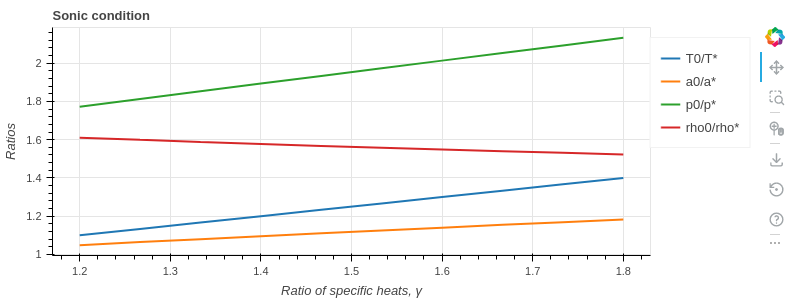
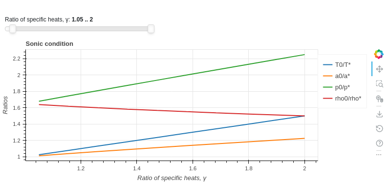
class pygasflow.interactive.diagrams.SonicDiagram(*, N, gamma_range, tooltips, _theme, _update_func, colors, error_log, figure, legend, show_legend_outside, show_minor_grid, size, title, x_label, x_range, y_label, y_range, name)

Plot the sonic conditions T0/T*=f(gamma), a0/a*=f(gamma), p0/p*=f(gamma), rho0/rhoT*=f(gamma).

Parameters:

figurebokeh.plotting._figure.figure

allow_None:

True

The Bokeh figure to populate

sizeTuple

allow_None:

True

default:

(800, 300)

length:

2

Size of the plot, (width, height) in pixel.

error_logString

default:

Visualize any error that raises from the computation.

colorsTuple

default:

(‘#1f77b4’, ‘#ff7f0e’, ‘#2ca02c’, ‘#d62728’, ‘#9467bd’, ‘#8c564b’, ‘#e377c2’, ‘#7f7f7f’, ‘#bcbd22’, ‘#17becf’)

length:

10

List of categorical colors.

legendbokeh.models.annotations.legends.Legend

allow_None:

True

The legend, when placed outside of the plotting area.

titleString

default:

x_labelString

default:

M

y_labelString

default:

Ratios

x_rangeRange

allow_None:

True

inclusive_bounds:

(True, True)

length:

2

y_rangeRange

allow_None:

True

inclusive_bounds:

(True, True)

length:

2

show_minor_gridBoolean

default:

False

Toggle minor grid visibility.

show_legend_outsideBoolean

default:

True

If True, the legend will be moved outside of the plotting area. In doing so, the legend items will become clickable, allowing user to hide a particular line.

gamma_rangeRange

bounds:

(1, 2)

default:

(1.05, 2)

inclusive_bounds:

(True, True)

length:

2

γ = Cp / Cv

NInteger

bounds:

N >= 10

default:

100

Number of points for each curve. It affects the quality of the visualization as well as the speed of updates.

tooltipsList

default:

[(‘Variable’, ‘@v’), (‘gamma’, ‘@xs’), (‘value’, ‘@ys’)]

Tooltips used on each line of the plot.

Examples

Show an interactive application:

from pygasflow.interactive.diagrams import SonicDiagram
SonicDiagram()

(Source code, large.png)

Set custom values to parameters and only show the figure:

from pygasflow.interactive.diagrams import SonicDiagram
d = SonicDiagram(gamma_range=(1.2, 1.8))
d.show_figure()

(Source code, large.png)

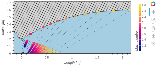
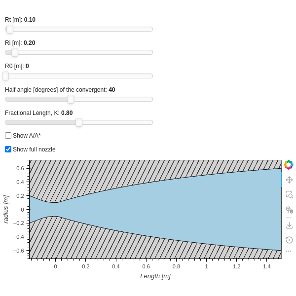
class pygasflow.interactive.diagrams.NozzleDiagram(*, characteristic_cmap, characteristic_scatter_kwargs, nozzle, show_area_ratio, show_characteristic_lines, show_divergent_only, show_full_nozzle, _theme, _update_func, colors, error_log, figure, legend, show_legend_outside, show_minor_grid, size, title, x_label, x_range, y_label, y_range, name)

Draw a representation of a nozzle.

Parameters:

figurebokeh.plotting._figure.figure

allow_None:

True

The Bokeh figure to populate

sizeTuple

allow_None:

True

default:

(800, 300)

length:

2

Size of the plot, (width, height) in pixel.

error_logString

default:

Visualize any error that raises from the computation.

colorsTuple

default:

(‘#1f77b4’, ‘#ff7f0e’, ‘#2ca02c’, ‘#d62728’, ‘#9467bd’, ‘#8c564b’, ‘#e377c2’, ‘#7f7f7f’, ‘#bcbd22’, ‘#17becf’)

length:

10

List of categorical colors.

legendbokeh.models.annotations.legends.Legend

allow_None:

True

The legend, when placed outside of the plotting area.

titleString

default:

x_labelString

default:

M

y_labelString

default:

Ratios

x_rangeRange

allow_None:

True

inclusive_bounds:

(True, True)

length:

2

y_rangeRange

allow_None:

True

inclusive_bounds:

(True, True)

length:

2

show_minor_gridBoolean

default:

False

Toggle minor grid visibility.

show_legend_outsideBoolean

default:

True

If True, the legend will be moved outside of the plotting area. In doing so, the legend items will become clickable, allowing user to hide a particular line.

nozzlepygasflow.nozzles.nozzle_geometry.Nozzle_Geometry

allow_None:

True

show_area_ratioBoolean

default:

False

If True show \(\frac{A}{A^{*}}\), otherwise shows the radius

show_full_nozzleBoolean

default:

False

If False, only show the positive y-coordinate.

show_divergent_onlyBoolean

default:

False

show_characteristic_linesBoolean

default:

False

Only used in MOC nozzles.

characteristic_scatter_kwargsDict

default:

{}

Rendering keywords for the scatter about characteristi lines.

characteristic_cmap(list, tuple, str)

allow_None:

True

A sequence of colors to use as the target palette for mapping.

This property can also be set as a String, to the name of any of the palettes shown in bokeh.palettes.

If not provided, colorcet.bmy will be used.

Examples

Show an interactive application:

from pygasflow.interactive.diagrams import NozzleDiagram
from pygasflow.nozzles import CD_TOP_Nozzle
nozzle = CD_TOP_Nozzle(Ri=0.2, Rt=0.1, Re=0.6, K=0.8)
NozzleDiagram(nozzle=nozzle, show_full_nozzle=True)

(Source code, large.png)

Set custom values to parameters and only show the figure:

from pygasflow.interactive.diagrams import NozzleDiagram
from pygasflow.nozzles import CD_Min_Length_Nozzle
nozzle = CD_Min_Length_Nozzle(Ri=0.3, Rt=0.2, Re=0.6)
d = NozzleDiagram(nozzle=nozzle, show_characteristic_lines=True)
d.show_figure()

(Source code, large.png)

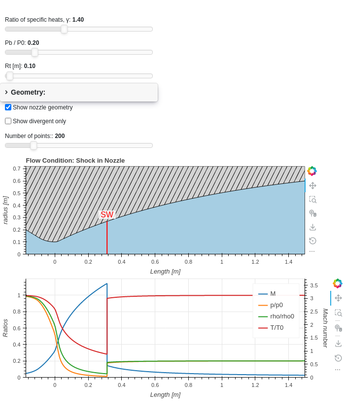
class pygasflow.interactive.diagrams.DeLavalDiagram(*, _show_all_ui_controls, labels, nozzle_diagram, show_nozzle, solver, tooltips, _theme, _update_func, colors, error_log, figure, legend, show_legend_outside, show_minor_grid, size, title, x_label, x_range, y_label, y_range, name)

Plot M, \(\frac{P}{P_{0}}\), \(\frac{T}{T_{0}}\), \(\frac{\rho}{\rho_{0}}\) along the length of a convergent-divergent nozzle.

Parameters:

figurebokeh.plotting._figure.figure

allow_None:

True

The Bokeh figure to populate

sizeTuple

allow_None:

True

default:

(800, 300)

length:

2

Size of the plot, (width, height) in pixel.

error_logString

default:

Visualize any error that raises from the computation.

colorsTuple

default:

(‘#1f77b4’, ‘#ff7f0e’, ‘#2ca02c’, ‘#d62728’, ‘#9467bd’, ‘#8c564b’, ‘#e377c2’, ‘#7f7f7f’, ‘#bcbd22’, ‘#17becf’)

length:

10

List of categorical colors.

legendbokeh.models.annotations.legends.Legend

allow_None:

True

The legend, when placed outside of the plotting area.

titleString

default:

x_labelString

default:

M

y_labelString

default:

Ratios

x_rangeRange

allow_None:

True

inclusive_bounds:

(True, True)

length:

2

y_rangeRange

allow_None:

True

inclusive_bounds:

(True, True)

length:

2

show_minor_gridBoolean

default:

False

Toggle minor grid visibility.

show_legend_outsideBoolean

default:

True

If True, the legend will be moved outside of the plotting area. In doing so, the legend items will become clickable, allowing user to hide a particular line.

solverpygasflow.solvers.de_laval.De_Laval_Solver

allow_None:

True

The solver instance.

tooltipsList

default:

[(‘Variable’, ‘@v’), (‘Length’, ‘@x’), (‘value’, ‘@y’)]

Tooltips used on each line of the plot.

labelsList

default:

[]

Labels to be used on the legend.

show_nozzleBoolean

default:

True

nozzle_diagrampygasflow.interactive.diagrams.nozzle.NozzleDiagram

allow_None:

True

The nozzle diagram instance to be shown.

Examples

Show an interactive application:

from pygasflow.interactive.diagrams import DeLavalDiagram
from pygasflow.nozzles import CD_TOP_Nozzle
from pygasflow.solvers import De_Laval_Solver
nozzle = CD_TOP_Nozzle(Ri=0.2, Rt=0.1, Re=0.6, K=0.8)
solver = De_Laval_Solver(
    gamma=1.4, R=287.05, T0=500, P0=101325,
    Pb_P0_ratio=0.2, nozzle=nozzle
)
DeLavalDiagram(solver=solver)

(Source code, large.png)

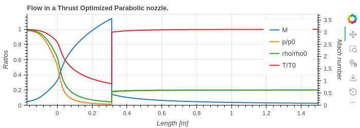
Only show the figure the solutions along the length of the nozzle:

from pygasflow.interactive.diagrams import DeLavalDiagram
from pygasflow.nozzles import CD_TOP_Nozzle
from pygasflow.solvers import De_Laval_Solver
nozzle = CD_TOP_Nozzle(Ri=0.2, Rt=0.1, Re=0.6, K=0.8)
solver = De_Laval_Solver(
    gamma=1.4, R=287.05, T0=500, P0=101325,
    Pb_P0_ratio=0.2, nozzle=nozzle
)
d = DeLavalDiagram(
    solver=solver,
    show_nozzle=False,
    title="Flow in a Thrust Optimized Parabolic nozzle."
)
d.show_figure()

(Source code, large.png)