Newtonian Flow Model
A few functions to quickly estimate the pressure distribution and the aerodynamic characteristics over the surfaces of simple geometric configurations with the Newtonian Theory.
Pressure Distribution
- pygasflow.atd.newton.pressure_coefficient(theta_b, alpha=0, beta=0, Mfs=None, gamma=1.4)[source]
Compute the pressure coefficient, Cp, with a Newtonian flow model.
There are four modes of operation:
Compute Cp with a Newtonian model:
pressure_coefficient(theta_b)Compute Cp with a modified Newtonian model:
pressure_coefficient(theta_b, Mfs=Mfs, gamma=gamma)Compute Cp with a Newtonian model for an axisymmetric configuration:
pressure_coefficient(theta_b, alpha=alpha, beta=beta)Compute Cp with a modified Newtonian model for an axisymmetric configuration:
pressure_coefficient(theta_b, alpha=alpha, beta=beta, Mfs=Mfs, gamma=gamma)
Note that for an axisymmetric configuration, the freestream flow does not impinge on those portions of the body surface which are inclined away from the freestream direction and which may, therefore, be thought of as lying in the “shadow of the freestream”.
- Parameters:
- theta_bfloat or array_like
Local body slope [radians]. Note that for a flat plate theta_b corresponds to the angle of attack.
- alphafloat or array_like, optional
Angle of attack [radians]. Default to 0 deg.
- betafloat or array_like, optional
Angular position of a point on the surface of the body [radians]. Default to 0 deg.
- Mfsfloat or array_like, optional
Free stream Mach number. Must be > 1.
- gammafloat or array_like, optional
Specific heats ratio. Default to 1.4. Must be \(\gamma > 1\).
- Returns:
- Cpfloat or array_like
Pressure coefficient.
References
“Basic of Aerothermodynamics”, by Ernst H. Hirschel
“Hypersonic Aerothermodynamics” by John J. Bertin
Examples
Compute Cp with a Newtonian model for a body with an angle of attack of 5deg:
>>> from pygasflow.atd.newton.pressures import pressure_coefficient
>>> from numpy import deg2rad
>>> pressure_coefficient(deg2rad(5))
np.float64(0.015192246987791938)
Compute Cp with a modified Newtonian model for a body with an angle of attack of 5deg with a free stream Mach number of 20 in air:
>>> pressure_coefficient(deg2rad(5), Mfs=20, gamma=1.4)
np.float64(0.01395744352416113)
Compute Cp with a Newtonian flow model for a sharp cone (axisymmetric configuration) with theta_b=15deg, exposed to an hypersonic stream of Helium with free stream Mach number of 14.9 and specific heat ratio 5/3, with an angle of attack of 10deg, at a point located beta=45deg:
>>> pressure_coefficient(deg2rad(15), alpha=deg2rad(10), beta=deg2rad(45))
np.float64(0.2789909245623247)
On the same axisymmetric configuration, compute Cp with a modified Netwonian flow mode:
>>> pressure_coefficient(deg2rad(15), alpha=deg2rad(10), beta=deg2rad(45), Mfs=14.9, gamma=5.0/3.0)
np.float64(0.2454586025665183)
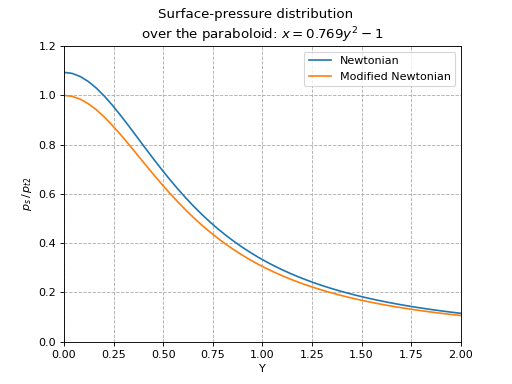
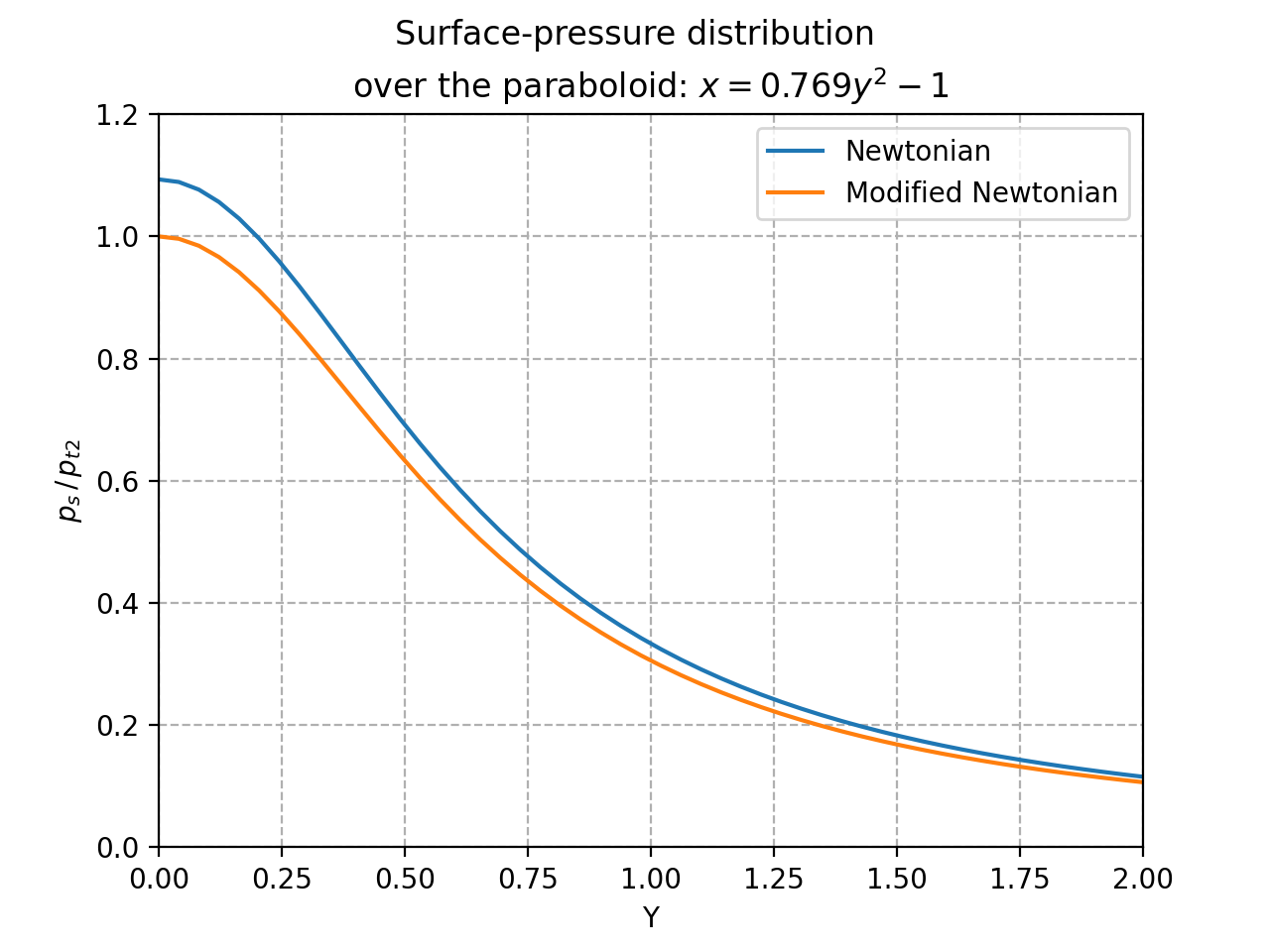
Compute the ratio ps / p_t2 using the Newtonian theory and the modified Newtonian theory, between the surface pressure, ps, and the total pressure behind a normal shockwave, p_t2, for the paraboloid
x = 0.769 * y**2 - 1. Use M_inf = 8 and gamma = 1.4. Note: this is a preproduction of Figure 3.9 of “Hypersonic and High-Temperature Gas Dynamics”, Third Edition, John D. Andersonfrom pygasflow import * from pygasflow.atd.newton import pressure_coefficient import numpy as np import matplotlib.pyplot as plt M_inf = 8 gamma = 1.4 a = 0.769 y = np.linspace(0, 2) # To get theta: rewrite the paraboloid in terms of y=f(x). # Find its tangent by differentiating it by x. Substitute x with the # paraboloid equation. Apply the arctan. theta = np.arctan(1 / (2 * a * np.sqrt(y**2))) Cp_newtonian = pressure_coefficient(theta) Cp_mod_newtonian = pressure_coefficient(theta, Mfs=M_inf, gamma=gamma) # from the definition of Cp ps_p_inf_newt = Cp_newtonian * M_inf**2 * gamma / 2 + 1 ps_p_inf_mod_newt = Cp_mod_newtonian * M_inf**2 * gamma / 2 + 1 # compute ratios across the shockwave shock = normal_shockwave_solver( "mu", M_inf, gamma=gamma, to_dict=True) # compute the flow quantities downstream of the normal shockwave flow2 = isentropic_solver("m", shock["md"], gamma=gamma, to_dict=True) p2_pt2 = 1 / flow2["pr"] # NOTE: alternatively, rayleigh_pitot_formula can be used pt2_p_inf = p2_pt2 * shock["pr"] # final results ps_pt2_newtonian = ps_p_inf_newt / pt2_p_inf ps_pt2_mod_newtonian = ps_p_inf_mod_newt / pt2_p_inf # plot plt.figure() plt.plot(y, ps_pt2_newtonian, label="Newtonian") plt.plot(y, ps_pt2_mod_newtonian, label="Modified Newtonian") plt.xlabel("Y") plt.ylabel(r"$p_{s} \, / \, p_{t2}$") plt.legend() plt.grid(which="major", visible=True, linestyle="--") plt.xlim(0, 2) plt.ylim(0, 1.2) plt.suptitle("Surface-pressure distribution") plt.title("over the paraboloid: $x = 0.769 y^{2} - 1$") plt.show()
(
Source code,png,hires.png,pdf)
- pygasflow.atd.newton.modified_newtonian_pressure_ratio(Mfs, theta_b, alpha=0, beta=0, gamma=1.4)[source]
Compute the pressure ratio \(\frac{P_{s}}{P_{t2}}\), between the static pressure in the shock layer and the pressure at the stagnation point.
- Parameters:
- Mfsfloat or array_like, optional
Free stream Mach number. Must be > 1.
- theta_bfloat or array_like
Local body slope [radians].
- alphafloat or array_like or None, optional
Angle of attack [radians]. Default to 0 deg.
- betafloat or array_like or None, optional
Angular position of a point on the surface of the body [radians]. Default to 0 deg.
- gammafloat or array_like, optional
Specific heats ratio. Default to 1.4. Must be \(\gamma > 1\).
- Returns:
- ps_pt2float or array_like
Ratio \(\frac{P_{s}}{P_{t2}}\).
References
“Hypersonic Aerothermodynamics” by John J. Bertin
Examples
Compute \(\frac{P_{s}}{P_{t2}}\) for a body with the following local body slope: [90deg, 60deg, 30deg, 0deg], immersed on a free stream with Mach number 10 having 0deg angle of attack:
>>> import numpy as np
>>> from pygasflow.atd.newton.pressures import modified_newtonian_pressure_ratio
>>> theta_b = np.deg2rad([90, 60, 30, 0])
>>> modified_newtonian_pressure_ratio(10, theta_b)
array([1.        , 0.75193473, 0.25580419, 0.00773892])
Compute \(\frac{P_{s}}{P_{t2}}\) for a body with the following local body slope: [90deg, 60deg, 30deg, 0deg], immersed on a free stream with Mach number 10 having 33deg angle of attack:
>>> theta_b = np.deg2rad([90, 60, 30, 0])
>>> modified_newtonian_pressure_ratio(10, theta_b, alpha=np.deg2rad(33))
array([0.70566393, 0.99728214, 0.79548767, 0.30207499])
- pygasflow.atd.newton.shadow_region(alpha, theta, beta=0)[source]
Compute the boundaries in the circumferential direction (
phi) in which the pressure coefficientCp=0for an axisymmetric object. The shadow region is identified by Cp<0.- Parameters:
- alphafloat or array_like
Angle of attack [radians].
- thetafloat or array_like
Local body slope [radians].
- betafloat or array_like
Sideslip angle [radians]. Default to 0 (no sideslip).
- Returns:
- phi_ifloat or array_like
Lower limit of the shadow region [radians]. If NaN, there is no shadow region.
- phi_ffloat or array_like
Upper limit of the shadow region [radians]. If NaN, there is no shadow region.
- funccallable
A lambda function with signature (alpha, theta, beta, phi), which can be used to test the configuration. It represents the angle between the velocity vector and the normal vector to the surface (see Notes).
Notes
The newtonian pressure coefficient is given by:
\(C_{p} = C_{p, t2} \cos^{2}{\eta}\)
where \(\cos{\eta}\) is the angle between the vecocity vector and and normal vector to the surface:
\(\cos{\eta} = \cos{\alpha} \cos{\beta} \sin{\theta} - \cos{\theta} \sin{\phi} \sin{\beta} - \cos{\phi} \cos{\theta} \sin{\alpha} \cos{\beta}\)
This function solves \(\cos{\eta} = 0\) for phi, the angle in the circumferential direction.
Let’s consider an axisymmetric geometry, for example a cone. The positive x-axis starts from the base and move to the apex. The base of the cone lies on the y-z plane, where the positive z-axis points down. The angle
phistarts from the negative z-axis and is positive in the counter-clockwise direction.| phi_i _|_ phi_f /\ | /\ / \|/ \ +y <-|---------|---- \ | / \ _|_ / | v +zThe pressure coefficient is positive for
phi_1 <= phi <= phi_f. The shadow region (where Cp<0) is identified by0 <= phi <= phi_1andphi_f <= phi <= 2 * pi.References
“Tables of aerodynamic coefficients obtained from developed newtonian expressions for complete and partial conic and spheric bodies at combined angle of attack and sideslip with some comparison with hypersonic experimental data”, by William R. Wells and William O. Armstrong, 1962.
Examples
>>> import numpy as np
>>> from pygasflow.atd.newton import shadow_region
>>> alpha = np.deg2rad(35)
>>> beta = np.deg2rad(0)
>>> theta_c = np.deg2rad(9)
>>> phi_i, phi_f, func = shadow_region(alpha, theta_c, beta)
>>> print(phi_i, phi_f)
1.342625208348352 4.940560098831234
- pygasflow.atd.newton.pressure_coefficient_tangent_cone(theta_c, gamma=1.4)[source]
Compute the pressure coefficient with the tangent-cone method.
- Parameters:
- theta_cfloat or array_like
Cone half-angle [radians].
- gammafloat, optional
Specific heats ratio. Default to 1.4. Must be \(\gamma > 1\).
- Returns:
- Cpfloat or array_like
Pressure coefficient
Examples
>>> from pygasflow.atd.newton.pressures import pressure_coefficient_tangent_cone
>>> from numpy import deg2rad
>>> pressure_coefficient_tangent_cone(deg2rad(10), 1.4)
np.float64(0.06344098329442194)
- pygasflow.atd.newton.pressure_coefficient_tangent_wedge(theta_w, gamma=1.4)[source]
Compute the pressure coefficient with the tangent-wedge method.
- Parameters:
- theta_wfloat or array_like
Wedge angle [radians].
- gammafloat, optional
Specific heats ratio. Default to 1.4. Must be \(\gamma > 1\).
- Returns:
- Cpfloat or array_like
Pressure coefficient
Examples
>>> from pygasflow.atd.newton.pressures import pressure_coefficient_tangent_wedge
>>> from numpy import deg2rad
>>> pressure_coefficient_tangent_wedge(deg2rad(10), 1.4)
np.float64(0.07310818074881005)
Aerodynamic Characteristics
- pygasflow.atd.newton.sharp_cone_solver(Rb, theta_c, alpha, beta=0, L=None, Cpt2=2, phi_1=0, phi_2=6.283185307179586, to_dict=None)[source]
Compute axial/normal/lift/drag/moments coefficients over a sharp cone or a slice.
- Parameters:
- Rbfloat or array_like
Radius of the base of the cone.
- theta_cfloat or array_like
Half-cone angle [radians].
- alphafloat or array_like
Angle of attack [radians].
- betafloat or array_like
Angle of sideslip [radians]. Default to 0 (no sideslip).
- LNone or float or array_like
Characteristic length to compute the moments. If None (default value) it will be set to Rb.
- Cpt2float or array_like, optional
Pressure coefficient at the stagnation point behind a shock wave. Default to 2 (newtonian theory).
- phi_1float
Initial angle of the slice. Default to 0 rad.
- phi_2float
Final angle of the slice. Default to 2*pi rad.
- to_dictbool, optional
Default value to False, which would return a tuple of results. If True, a dictionary will be returned, whose keys are listed in the Returns section.
- Returns:
- CNfloat or array_like
Normal force coefficient.
- CAfloat or array_like
Axial force coefficient.
- CYfloat or array_like
Side-force coefficient.
- CLfloat or array_like
Lift coefficient.
- CDfloat or array_like
Drag coefficient.
- CSfloat or array_like
Crosswind coefficient.
- L/Dfloat or array_like
Lift/Drag ratio.
- Clfloat or array_like
Rolling-moment coefficient.
- Cmfloat or array_like
Pitching-moment coefficient.
- Cnfloat or array_like
Yawing-moment coefficient.
See also
pressure_coefficient,sphere_solver
Notes
The reference system is:
-z | | y --------- /| / | / | x / | zphi_1andphi_2are the angles starting from the -z axis, rotating counter-clockwise.References
“Tables of aerodynamic coefficients obtained from developed newtonian expressions for complete and partial conic and spheric bodies at combined angle of attack and sideslip with some comparison with hypersonic experimental data”, by William R. Wells and William O. Armstrong, 1962.
Hypersonic Aerothermodynamics, John J. Bertin
Examples
Compute the aerodynamic characteristics for a sharp cone having radius 1, for different angle of attacks with no sideslip:
>>> import numpy as np
>>> from pygasflow.atd.newton.sharp_cone import sharp_cone_solver
>>> theta_c = np.deg2rad(10)
>>> alpha = np.linspace(0, np.pi)
>>> beta = np.deg2rad(0)
>>> res = sharp_cone_solver(1, theta_c, alpha, beta, to_dict=True)
Compute the aerodynamic characteristics for a slice of sharp cone with
phi_1=90 degandphi_2=270 deg:>>> res = sharp_cone_solver(1, theta_c, alpha, beta, to_dict=True, ... phi_1=np.pi/2, phi_2=1.5*np.pi)
- pygasflow.atd.newton.lift_drag_crosswind(CA, CY, CN, alpha, beta=0)[source]
Compute the lift, drag and crosswind coefficients in the wind frame starting from the axial, side force, normal coefficients in the body frame.
- Parameters:
- CA, CY, CNarray_like
Axial, Side force and Normal coefficients in the body frame.
- alphaarray_like
Angle of attack [radians].
- betaarray_like
Side slip angle [radians]. Default to 0 (no sideslip).
- Returns:
- CL, CD, CSarray_like
Lift, Drag and Crosswind coefficients in the wind frame.